【图像分类案例】(8) ResNet50 鸟类图像4分类，附Pytorch完整代码_鸟类分类代码

大家好，今天和大家分享一些如何使用 Pytorch 搭建 ResNet50 卷积神经网络模型，并使用迁移学习的思想训练网络，完成鸟类图片的预测。

ResNet 的原理 和 TensorFlow2 实现方式可以看我之前的两篇博文，这里就不详细说明原理了。

ResNet18、34： https://blog.csdn.net/dgvv4/article/details/122396424

ResNet50： https://blog.csdn.net/dgvv4/article/details/121878494

---

1. 模型构建

首先导入网络构建过程中所有需要用到的工具包，本小节的所有代码写在 ResNet.py 文件中

import torch
from torch import nn
from torchstat import stat  # 查看网络参数
from torchsummary import summary  # 查看网络结构

1.1 构建单个残差块

残差单元的结构如下图所示，一种是基本模块，即输入特征图的尺寸和输出特征层的尺寸相同，两个特征图可以直接叠加；一种是下采样模块，即主干部分对输入特征图使用 stride=2 的下采样卷积，使得输入特征图的尺寸变成原来的一半，那么残差边部分也需要对输入特征图进行下采样操作，使得输入特征图经过残差边处理后的 shape 能和主干部分处理后的特征图 shape 相同，从而能够将残差边输出和主干输出直接叠加。

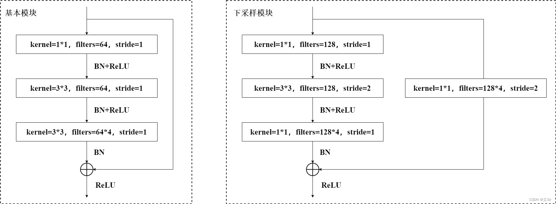
以下图基本残差块为例，先对输入图像使用 1*1 卷积下降通道数，在低维空间下使用 3*3 卷积提取特征，然后再使用 1*1 卷积上升通道数，残差连接输入和输出，将叠加后的结果进过 relu 激活函数。

代码如下：

# -------------------------------------------- #
#（1）残差单元
# x--> 卷积 --> bn --> relu --> 卷积 --> bn --> 输出 
# |---------------Identity(短接)----------------|
'''
in_channel   输入特征图的通道数 
out_channel  第一次卷积输出特征图的通道数
stride=1     卷积块中3*3卷积的步长
downsample   是否下采样
'''
# -------------------------------------------- #
class Bottleneck(nn.Module):
    # 最后一个1*1卷积下降的通道数
    expansion = 4
    
    # 初始化
    def __init__(self, in_channel, out_channel, stride=1, downsample=None):
        # 继承父类初始化方法
        super(Bottleneck, self).__init__()
        
        # 属性分配
        # 1*1卷积下降通道，padding='same'，若stride=1，则[b,in_channel,h,w]==>[b,out_channel,h,w]
        self.conv1 = nn.Conv2d(in_channels=in_channel, out_channels=out_channel,
                               kernel_size=1, stride=1, padding=0, bias=False)
 
        # BN层是计算特征图在每个channel上面的均值和方差，需要给出输出通道数
        self.bn1 = nn.BatchNorm2d(out_channel)
        
        # relu激活, inplace=True节约内存
        self.relu = nn.ReLU(inplace=True)
        
        # 3*3卷积提取特征，[b,out_channel,h,w]==>[b,out_channel,h,w]
        self.conv2 = nn.Conv2d(in_channels=out_channel, out_channels=out_channel,
                               kernel_size=3, stride=stride, padding=1, bias=False)
        
        # BN层, 有bn层就不需要bias偏置
        self.bn2 = nn.BatchNorm2d(out_channel)
        
        # 1*1卷积上升通道 [b,out_channel,h,w]==>[b,out_channel*expansion,h,w]
        self.conv3 = nn.Conv2d(in_channels=out_channel, out_channels=out_channel*self.expansion,
                               kernel_size=1, stride=1, padding=0, bias=False)
        
        # BN层，对out_channel*expansion标准化
        self.bn3 = nn.BatchNorm2d(out_channel*self.expansion)
        
        # 记录是否需要下采样, 下采样就是第一个卷积层的步长=2，输入和输出的图像的尺寸不一致
        self.downsample = downsample
    
    # 前向传播
    def forward(self, x):
        
        # 残差边
        identity = x
        
        # 如果第一个卷积层stride=2下采样了，那么残差边也需要下采样
        if self.downsample is not None:
            # 下采样方法
            identity = self.downsample(x)
        
        # 主干部分
        x = self.conv1(x)
        x = self.bn1(x)
        x = self.relu(x)
        
        x = self.conv2(x)
        x = self.bn2(x)
        x = self.relu(x)
        
        x = self.conv3(x)
        x = self.bn3(x)
        
        # 残差连接
        x = x + identity
        # relu激活
        x = self.relu(x)
        
        return x  # 输出残差单元的结果

---

1.2 构建网络

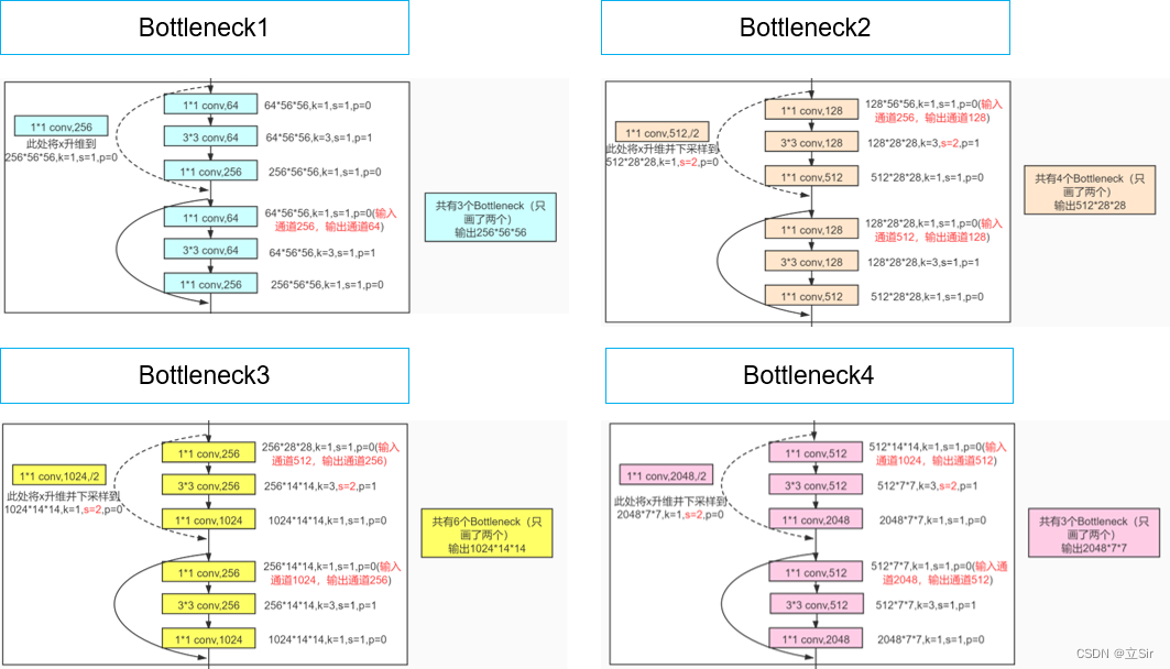
我们已经成功构建完单个残差单元的类，而残差结构就是由多个残差单元堆叠而来的，ResnNet50 中有 4 组残差结构，每个残差结构分别堆叠了 3，4，6，3 个残差单元，如下图所示。

第一个残差结构中的第一个残差单元只需要调整输入特征图的通道数，不需要改变特征图的尺寸；而其他三个的残差结构的第一个残差单元不仅需要对输入特征图调整通道数，还要对输入特征图进行下采样操作。

代码如下：

# -------------------------------------------- #
#（2）网络构建
'''
block： 残差单元
blocks_num： 每个残差结构使用残差单元的数量
num_classes： 分类数量
include_top： 是否包含分类层（全连接）
'''
# -------------------------------------------- #
class ResNet(nn.Module):
    # 初始化
    def __init__(self, block, blocks_num, num_classes=1000, include_top=True):
        # 继承父类初始化方法
        super(ResNet, self).__init__()
        
        # 属性分配
        self.include_top = include_top
        self.in_channel = 64  # 第一个卷积层的输出通道数
        
        # 7*7卷积下采样层处理输入图像 [b,3,h,w]==>[b,64,h,w]
        self.conv1 = nn.Conv2d(in_channels=3, out_channels=self.in_channel, 
                               kernel_size=7, stride=2, padding=3, bias=False)
        
        # BN对每个通道做标准化
        self.bn1 = nn.BatchNorm2d(self.in_channel)
        
        # relu激活函数
        self.relu = nn.ReLU(inplace=True)
        
        # 3*3最大池化层 [b,64,h,w]==>[b,64,h//2,w//2]
        self.maxpool = nn.MaxPool2d(kernel_size=3, stride=2, padding=1)
        
        # 残差卷积块
        # 第一个残差结构不需要下采样只需要调整通道
        self.layer1 = self._make_layer(block, 64, blocks_num[0])
        # 下面的残差结构的第一个残差单元需要进行下采样
        self.layer2 = self._make_layer(block, 128, blocks_num[1], stride=2)     
        self.layer3 = self._make_layer(block, 256, blocks_num[2], stride=2)       
        self.layer4 = self._make_layer(block, 512, blocks_num[3], stride=2)
        
        # 分类层
        if self.include_top:
            # 自适应全局平均池化，无论输入特征图的shape是多少，输出特征图的(h,w)==(1,1)
            self.avgpool = nn.AdaptiveAvgPool2d((1,1))  # output
            # 全连接分类
            self.fc = nn.Linear(512*block.expansion, num_classes)
        
        # 卷积层权重初始化
        for m in self.modules():
            if isinstance(m, nn.Conv2d):
                nn.init.kaiming_normal_(m.weight, mode='fan_out')
        
    # 残差结构
    '''
    block: 代表残差单元
    channel: 残差结构中第一个卷积层的输出通道数
    block_num: 代表一个残差结构包含多少个残差单元
    stride: 是否下采样stride=2
    '''
    def _make_layer(self, block, channel, block_num, stride=1):
        
        # 是否需要进行下采样
        downsample = None
        
        # 如果stride=2或者残差单元的输入和输出通道数不一致
        # 就对残差单元的shortcut部分执行下采样操作
        if stride != 1 or self.in_channel != channel * block.expansion:
            
            # 残差边需要下采样
            downsample = nn.Sequential(
                # 对于第一个残差单元的残差边部分只需要调整通道
                nn.Conv2d(in_channels=self.in_channel, out_channels=channel*block.expansion, 
                          kernel_size=1, stride=stride, bias=False),
                nn.BatchNorm2d(channel*block.expansion))
 
        # 一个残差结构堆叠多个残差单元
        layers = []
        # 先堆叠第一个残差单元，因为这个需要下采样
        layers.append(block(self.in_channel, channel, stride=stride, downsample=downsample))
        
        # 获得第一个残差单元的输出特征图个数, 作为第二个残差单元的输入
        self.in_channel = channel * block.expansion
        
        # 堆叠剩下的残差单元，此时的shortcut部分不需要下采样
        for _ in range(1, block_num):
            layers.append(block(self.in_channel, channel))
 
        # 返回构建好了的残差结构
        return nn.Sequential(*layers)  # *代表将layers以非关键字参数的形式返还
 
    # 前向传播
    def forward(self, x):
        # 输入层
        x = self.conv1(x)
        x = self.bn1(x)
        x = self.relu(x)
        x = self.maxpool(x)
        
        # 残差结构
        x = self.layer1(x)
        x = self.layer2(x)
        x = self.layer3(x)
        x = self.layer4(x)
        
        # 分类层
        if self.include_top:
            # 全局平均池化
            x = self.avgpool(x)
            # 打平
            x = torch.flatten(x, 1)
            # 全连接分类
            x = self.fc(x)
        
        return x

---

1.3 查看网络结构

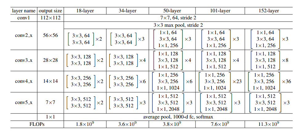
 [3,4,6,3] 代表四个残差结构中分别堆叠了多少个残差单元，include_top=True 代表包含网络的分类层，默认是1000个分类，即全连接层输出预测结果。网络结构如下图所示：

# 构建resnet50
def resnet50(num_classes=1000, include_top=True):
    return  ResNet(Bottleneck, [3,4,6,3], num_classes=num_classes, include_top=include_top)
 
 
if __name__ == '__main__':
    
    # 接收网络模型
    model = resnet50()
    # print(model)
    
    # 查看网络参数量，不需要指定输入特征图像的batch维度
    stat(model, input_size=(3,224,224))
    
    # 查看网络结构及参数
    summary(model, input_size=[(3,224,224)], device='cpu')

网络的参数量和计算量如下：

================================================================
Total params: 25,557,032
Trainable params: 25,557,032
Non-trainable params: 0
----------------------------------------------------------------
Input size (MB): 0.57
Forward/backward pass size (MB): 286.56
Params size (MB): 97.49
Estimated Total Size (MB): 384.62
----------------------------------------------------------------

---

2. 网络训练

2.1 文件配置

首先我们需要将接下来所有用到的文件包，文件路径，先写好了方便统一管理。使用迁移学习的方法训练网络。

import torch
from torch import nn, optim
from torchvision import datasets, transforms
from torch.utils.data import DataLoader
from ResNet import resnet50  # 从自定义的ResNet.py文件中导入resnet50这个函数
import numpy as np
import matplotlib.pyplot as plt
 
# -------------------------------------------------- #
#（0）参数设置
# -------------------------------------------------- #
batch_size = 32  # 每个step训练32张图片
epochs = 10  # 共训练10次
 
# -------------------------------------------------- #
#（1）文件配置
# -------------------------------------------------- #
# 数据集文件夹位置
filepath = 'D:/deeplearning/test/数据集/4种鸟分类/new_data/'
# 权重文件位置
weightpath = 'D:/deeplearning/imgnet/pytorchimgnet/pretrained_weights/resnet50.pth'
# 权重保存文件夹路径
savepath = 'D:/deeplearning/imgnet/pytorchimgnet/save_weights/'
 
# 获取GPU设备
if torch.cuda.is_available():  # 如果有GPU就用，没有就用CPU
    device = torch.device('cuda:0')
else:
    device = torch.device('cpu')

---

2.2 构造数据集

首先定义训练集和验证集的数据预处理函数。将输入图像的尺寸变成模型要求的 224*224 大小，然后再将像素值类型从 numpy 变成 tensor 类型，并归一化处理，像素值大小从 [0,255] 变换到 [0,1]，再调整输入图像的维度，从 [h,w,c] 变成 [c,h,w]；接着对图像的每个颜色通道做标准化处理，使像素值满足以0.5为均值，0.5为方差的正态分布。

预处理之后就构造训练集和验证集，指定 batch_size=32，代表训练时每个 step 训练32张图片

# -------------------------------------------------- #
#（2）构造数据集
# -------------------------------------------------- #
# 训练集的数据预处理
transform_train = transforms.Compose([
    # 数据增强，随机裁剪224*224大小
    transforms.RandomResizedCrop(224),
    # 数据增强，随机水平翻转
    transforms.RandomHorizontalFlip(),
    # 数据变成tensor类型，像素值归一化，调整维度[h,w,c]==>[c,h,w]
    transforms.ToTensor(),
    # 对每个通道的像素进行标准化，给出每个通道的均值和方差
    transforms.Normalize(mean=(0.5,0.5,0.5), std=(0.5,0.5,0.5))])
 
# 验证集的数据预处理
transform_val = transforms.Compose([
    # 将输入图像大小调整为224*224
    transforms.Resize((224,224)),
    transforms.ToTensor(),
    transforms.Normalize(mean=(0.5,0.5,0.5), std=(0.5,0.5,0.5))])
 
# 读取训练集并预处理
train_dataset = datasets.ImageFolder(root=filepath + 'train',  # 训练集图片所在的文件夹
                                     transform = transform_train)  # 训练集的预处理方法
 
# 读取验证集并预处理
val_dataset = datasets.ImageFolder(root=filepath + 'val',  # 验证集图片所在的文件夹
                                     transform = transform_val)  # 验证集的预处理方法
 
# 查看训练集和验证集的图片数量
train_num = len(train_dataset)
val_num = len(val_dataset)
print('train_num:', train_num, 'val_num:', val_num)   # 453, 112
 
# 查看图像类别及其对应的索引
class_dict = train_dataset.class_to_idx
print(class_dict)  # {'Bananaquit': 0, 'Black Skimmer': 1, 'Black Throated Bushtiti': 2, 'Cockatoo': 3}
# 将类别名称保存在列表中
class_names = list(class_dict.keys())
 
# 构造训练集
train_loader = DataLoader(dataset=train_dataset,  # 接收训练集
                          batch_size=batch_size,  # 训练时每个step处理32张图
                          shuffle=True,           # 打乱每个batch
                          num_workers=0)          # 加载数据时的线程数量，windows环境下只能=0
 
# 构造验证集
val_loader = DataLoader(dataset=val_dataset,
                        batch_size=batch_size,
                        shuffle=False,
                        num_workers=0)

---

2.3 数据可视化

接下来查看一下数据集中构造的图片和标签是什么样的，这里要注意的是在预处理时已经对整个数据集做了归一化和以 0.5 为均值 0.5 为方差做的标准化。这里需要做一次反标准化，img = img / 2 + 0.5，变会归一化之后的结果。不然画出来的图太抽象了。

标准化：         反标准化： 

# -------------------------------------------------- #
#（3）数据可视化
# -------------------------------------------------- #
# 取出一个batch的训练集，返回图片及其标签
train_img, train_label = iter(train_loader).next()
# 查看shape, img=[32,3,224,224], label=[32]
print(train_img.shape, train_label.shape)
 
# 从一个batch中取出前9张图片
img = train_img[:9]  # [9, 3, 224, 224]
# 将图片反标准化，像素变到0-1之间
img = img / 2 + 0.5
# tensor类型变成numpy类型
img = img.numpy()
class_label = train_label.numpy()
# 维度重排 [b,c,h,w]==>[b,h,w,c]
img = np.transpose(img, [0,2,3,1])
 
# 创建画板
plt.figure()
# 绘制四张图片
for i in range(img.shape[0]):
    plt.subplot(3,3,i+1)
    plt.imshow(img[i])
    plt.xticks([])  # 不显示x轴刻度
    plt.yticks([])  # 不显示y轴刻度
    plt.title(class_names[class_label[i]])  # 图片对应的类别
 
plt.tight_layout()  # 轻量化布局
plt.show()

绘制前9张图片及其标签：

---

2.4 模型构建

首先导入我们构建的 resnet50 网络模型，它默认有 1000 个分类，也就是网络的最后一个全连接层的输出结果和我们当前的任务不一样。

通过 torch.load() 将权重文件加载到内存中，再通过 net.load_state_dict() 将网络的每一层权重加载上来。此时的全连接层是1000分类，因此我们将它修改为4分类的，通过 net.fc.in_features 获取最后一个全连接层的输入通道数，然后再重写这个全连接层 net.fc = nn.Linear(in_channel, 4) 将其输出神经元个数改成4个。

# -------------------------------------------------- #
#（4）加载模型
# -------------------------------------------------- #
# 1000分类层
net = resnet50(num_classes=1000, include_top=True)
 
# 加载预训练权重
net.load_state_dict(torch.load(weightpath, map_location=device))
 
# 为网络重写分类层
in_channel = net.fc.in_features  # 2048
net.fc = nn.Linear(in_channel, 4)  # [b,2048]==>[b,4]
 
# 将模型搬运到GPU上
net.to(device)
# 定义交叉熵损失
loss_function = nn.CrossEntropyLoss()
# 定义优化器
optimizer = optim.Adam(net.parameters(), lr=0.002)
 
# 保存准确率最高的一次迭代
best_acc = 0.0

---

2.5 训练与验证

这里要注意的就是网络训练和测试的模式不一样，训练时 Dropout 层随机杀死神经元，BN层计算在 batch 维度上计算均值和方差；验证时 Dropout 层不起作用，BN 层去整个训练集计算得到的均值和方差。通过 net.train() 和 net.eval() 来切换训练和验证模式。

# -------------------------------------------------- #
#（5）网络训练
# -------------------------------------------------- #
for epoch in range(epochs):
    
    print('-'*30, '\n', 'epoch:', epoch)
    
    # 将模型设置为训练模型, dropout层和BN层只在训练时起作用
    net.train()
    
    # 计算训练一个epoch的总损失
    running_loss = 0.0
    
    # 每个step训练一个batch
    for step, data in enumerate(train_loader):
        # data中包含图像及其对应的标签
        images, labels = data
        
        # 梯度清零，因为每次计算梯度是一个累加
        optimizer.zero_grad()
        
        # 前向传播
        outputs = net(images.to(device))
        
        # 计算预测值和真实值的交叉熵损失
        loss = loss_function(outputs, labels.to(device))
        
        # 梯度计算
        loss.backward()
        
        # 权重更新
        optimizer.step()
        
        # 累加每个step的损失
        running_loss += loss.item()
        
        # 打印每个step的损失
        print(f'step:{step} loss:{loss}')
    
    
# -------------------------------------------------- #
#（6）网络验证
# -------------------------------------------------- #
    net.eval()  # 切换为验证模型，BN和Dropout不起作用
    
    acc = 0.0   # 验证集准确率
    
    with torch.no_grad():  # 下面不进行梯度计算
        
        # 每次验证一个batch
        for data_test in val_loader:
            
            # 获取验证集的图片和标签
            test_images, test_labels = data_test
            
            # 前向传播
            outputs = net(test_images.to(device))
            
            # 预测分数的最大值
            predict_y = torch.max(outputs, dim=1)[1]
            
            # 累加每个step的准确率
            acc += (predict_y == test_labels.to(device)).sum().item()
            
        # 计算所有图片的平均准确率
        acc_test = acc / val_num
        
        # 打印每个epoch的训练损失和验证准确率
        print(f'total_train_loss:{running_loss/step}, total_test_acc:{acc_test}')
 
        
# -------------------------------------------------- #
#（7）权重保存
# -------------------------------------------------- #
        # 保存最好的准确率的权重
        if acc_test > best_acc:
            # 更新最佳的准确率
            best_acc = acc_test
            # 保存的权重名称
            savename = savepath + 'resnet50.pth'
            # 保存当前权重
            torch.save(net.state_dict(), savename)

训练过程如下：

------------------------------ 
 epoch: 9
step:0 loss:0.6036051511764526
step:1 loss:0.9885318279266357
step:2 loss:0.5862273573875427
step:3 loss:0.5116483569145203
step:4 loss:0.5162124633789062
step:5 loss:0.5078244805335999
step:6 loss:0.40748751163482666
step:7 loss:0.477965384721756
step:8 loss:0.5453536510467529
step:9 loss:0.4567239284515381
step:10 loss:0.28334566950798035
step:11 loss:0.4871848225593567
step:12 loss:0.47422197461128235
step:13 loss:0.5443617105484009
step:14 loss:0.5486546754837036
total_train_loss:0.5670963547059468, total_test_acc:0.8660714285714286

---

3. 预测阶段

3.1 文件配置

首先将工具包和文件路径先写好，便于统一管理

import torch
from torchvision import transforms
from PIL import Image
from ResNet import resnet50
import matplotlib.pyplot as plt
 
# -------------------------------------------------- #
#（0）参数设置
# -------------------------------------------------- #
# 图片文件路径
img_path = 'D:/deeplearning/imgnet/pytorchimgnet/img/Black_Throated_Bushtiti.jpg'
# 权重参数路径
weights_path = 'D:/deeplearning/imgnet/pytorchimgnet/save_weights/resnet50.pth'
# 预测索引对应的类别名称
class_names=['Bananaquit', 'Black Skimmer', 'Black Throated Bushtiti', 'Cockatoo']
 
# 获取GPU设备
if torch.cuda.is_available():  # 如果有GPU就用，没有就用CPU
    device = torch.device('cuda:0')
else:
    device = torch.device('cpu')

---

3.2 数据预处理和可视化

这里采用和验证集相同的预处理方法，由于只预测一张图像，因此在送入网络之前需要给图像增加 batch 维度，[c,h,w]==>[b,c,h,w]

# -------------------------------------------------- #
#（1）数据加载
# -------------------------------------------------- #
# 预处理函数
data_transform = transforms.Compose([
    # 将输入图像的尺寸变成224*224
    transforms.Resize((224,224)),
    # 数据变成tensor类型，像素值归一化，调整维度[h,w,c]==>[c,h,w]
    transforms.ToTensor(),
    # 对每个通道的像素进行标准化，给出每个通道的均值和方差
    transforms.Normalize(mean=(0.5,0.5,0.5), std=(0.5,0.5,0.5))])
 
# 读取图片
frame = Image.open(img_path)
# 展示图片
plt.imshow(frame)
plt.title('Black_Throated_Bushtiti')
plt.show()
 
# 数据预处理
img = data_transform(frame)
# 给图像增加batch维度 [c,h,w]==>[b,c,h,w]
img = torch.unsqueeze(img, dim=0)

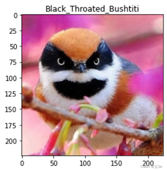
需要预测的图像及其标签

---

3.3 图片预测

在网络前向传播之前将模型设置为验证模式 model.eval()，只做前向传播的操作，不进行梯度更新操作 with torch.no_grad(): 不计算梯度。

经过前向传播后，图像的shape变成 [b,4]，由于这里的 batch_size=1，因此将可以将batch维度挤压掉，得到由4个元素组成的向量，代表图片属于四个类别的分数。

# -------------------------------------------------- #
#（2）图像预测
# -------------------------------------------------- #
# 加载模型
model = resnet50(num_classes=4, include_top=True)
# 加载权重文件
model.load_state_dict(torch.load(weights_path, map_location=device))
# 模型切换成验证模式，dropout和bn切换形式
model.eval()
 
# 前向传播过程中不计算梯度
with torch.no_grad():
    # 前向传播
    outputs = model(img)
    # 只有一张图就挤压掉batch维度
    outputs = torch.squeeze(outputs)
    # 计算图片属于4个类别的概率
    predict = torch.softmax(outputs, dim=0)
    # 得到类别索引
    predict_cla = torch.argmax(predict).numpy()
 
# 获取最大预测类别概率
predict_score = round(torch.max(predict).item(), 4)
# 获取预测类别的名称
predict_name = class_names[predict_cla]
 
# 展示预测结果
plt.imshow(frame)
plt.title('class: '+str(predict_name)+'\n score: '+str(predict_score))
plt.show()

预测结果如图：