Python纯手动搭建BP神经网络（手写数字识别）_填写digit_predict(train_sample, train_label, test_sa

来源：投稿 作者：张宇
编辑：学姐

 

实验介绍

实验要求：

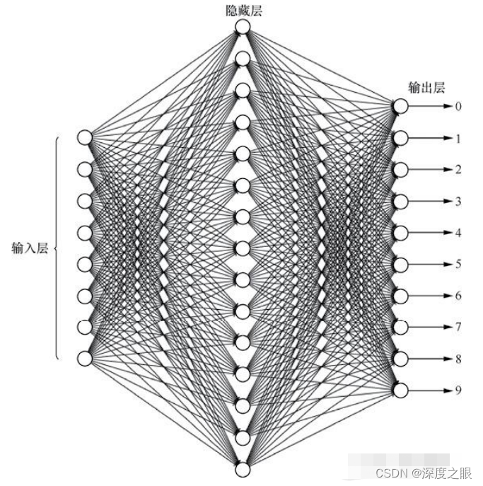
实现一个手写数字识别程序，如下图所示，要求神经网络包含一个隐层，隐层的神经元个数为15。

整体思路：

主要参考西瓜书第五章神经网络部分的介绍，使用批量梯度下降对神经网络进行训练。

读取并处理数据

数据读取思路：

• 数据集中给出的图片为28*28的灰度图，利用 plt.imread() 函数将图片读取出来后为 28x28 的数组，如果使用神经网络进行训练的话，我们可以将每一个像素视为一个特征，所以将图片利用numpy.reshape 方法将图片化为 1x784 的数组。读取全部数据并将其添加进入数据集 data 内，将对应的标签按同样的顺序添加进labels内。

• 然后使用np.random.permutation方法将索引打乱，利用传入的测试数据所占比例test_ratio将数据划分为测试集与训练集。

• 使用训练样本的均值和标准差对训练数据、测试数据进行标准化。标准化这一步很重要，开始忽视了标准化的环节，神经网络精度一直达不到效果。

• 返回数据集

这部分代码如下：

# 读取图片数据 参数：数据路径 测试集所占的比例
def loadImageData(trainingDirName='data/', test_ratio=0.3):
    from os import listdir
    data = np.empty(shape=(0, 784))
    labels = np.empty(shape=(0, 1))
 
    for num in range(10):
        dirName = trainingDirName + '%s/' % (num)  # 获取当前数字文件路径
        # print(listdir(dirName))
        nowNumList = [i for i in listdir(dirName) if i[-3:] == 'bmp']  # 获取里面的图片文件
        labels = np.append(labels, np.full(shape=(len(nowNumList), 1), fill_value=num), axis=0)  # 将图片标签加入
        for aNumDir in nowNumList:  # 将每一张图片读入
            imageDir = dirName + aNumDir  # 构造图片路径
            image = plt.imread(imageDir).reshape((1, 784))  # 读取图片数据
            data = np.append(data, image, axis=0)  
    # 划分数据集
    m = data.shape[0]
    shuffled_indices = np.random.permutation(m)  # 打乱数据
    test_set_size = int(m * test_ratio)
    test_indices = shuffled_indices[:test_set_size]
    train_indices = shuffled_indices[test_set_size:]
 
    trainData = data[train_indices]
    trainLabels = labels[train_indices]
 
    testData = data[test_indices]
    testLabels = labels[test_indices]
 
    # 对训练样本和测试样本使用统一的均值 标准差进行归一化
    tmean = np.mean(trainData)
    tstd = np.std(testData)
 
    trainData = (trainData - tmean) / tstd
    testData = (testData - tmean) / tstd
    return trainData, trainLabels, testData, testLabels

OneHot编码：

由于神经网络的特性，在进行多分类任务时，每一个神经元的输出对应于一个类，所以将每一个训练样本的标签转化为OneHot形式（将0-9的数据映射在长度为10的向量中，每个样本向量对应位置的值为1其余为0）。

# 对输出标签进行OneHot编码  参数：labels 待编码的标签  Label_class  编码类数
def OneHotEncoder(labels,Label_class):
    one_hot_label = np.array([[int(i == int(labels[j])) for i in range(Label_class)] for j in range(len(labels))])
    return one_hot_label
 

训练神经网络

激活函数：

激活函数使用sigmoid函数，但是使用定义式在训练过程中总是出现 overflow 警告，所以将函数进行了如下形式的转化。

# sigmoid激活函数
def sigmoid(z):
    for r in range(z.shape[0]):
        for c in range(z.shape[1]):
            if z[r,c] >= 0:
                z[r,c] = 1 / (1 + np.exp(-z[r,c]))
            else :
                z[r,c] = np.exp(z[r,c]) / (1 + np.exp(z[r,c]))
    return z

损失函数：

使用均方误差损失函数。其实我感觉在这个题目里面直接使用预测精度也是可以的。

def cost(prediction, labels):
    return np.mean(np.power(prediction - labels,2))

训练：

终于来到了紧张而又刺激的训练环节。神经网络从输入层通过隐层传递的输出层进而获得网络的输出叫做正向传播，而从输出层根据梯度下降的方法进行调整权重及偏置的过程叫做反向传播。

前向传播每层之间将每个结点的输出值乘对应的权重（对应函数中 omega1 omega2 ）传输给下一层结点，下一层结点将上一层所有传来的数据进行求和，并减去偏置 theta （此时数据对应函数中 h_in o_in ）。最后通过激活函数输出下一层（对应函数中 h_out o_out ）。在前向传播完成后计算了一次损失，方便后面进行分析。

反向传播是用梯度下降法对权重和偏置进行更新，这里是最主要的部分。根据西瓜书可以推出输出层权重的调节量为 ,其中 为学习率， 分别为对应数据的真实值以及网络的输出， 为隐层的输出值。这里还要一个重要的地方在于如果将公式向量化的话需要重点关注输出矩阵形状以及每个矩阵数据之间的关系。代码中d2 对应于公式中 这一部分，这里需要对应值相乘。最后将这一部分与进行矩阵乘法，在乘学习率得到权重调节量，与权重相加即可（代码中除了训练集样本个数m是因为 d2 与 h_out 的乘积将所有训练样本进行了累加，所以需要求平均）。

对于其他权重及偏置的调节方式与此类似，不做过多介绍（其实是因为明天要上课，太晚了得睡觉，有空补上这里和其他不详细的地方），详见西瓜书。

# 训练一轮ANN 参数：训练数据 标签 输入层 隐层 输出层size 输入层隐层连接权重 隐层输出层连接权重 偏置1  偏置2 学习率
def trainANN(X, y, input_size, hidden_size, output_size, omega1, omega2, theta1, theta2, learningRate):
    # 获取样本个数
    m = X.shape[0]
    # 将矩阵X,y转换为numpy型矩阵
    X = np.matrix(X)
    y = np.matrix(y)
 
    # 前向传播 计算各层输出
    # 隐层输入 shape=m*hidden_size
    h_in = np.matmul(X, omega1.T) - theta1.T
    # 隐层输出 shape=m*hidden_size
    h_out = sigmoid(h_in)
    # 输出层的输入 shape=m*output_size
    o_in = np.matmul(h_out, omega2.T) - theta2.T
    # 输出层的输出 shape=m*output_size
    o_out = sigmoid(o_in)
 
    # 当前损失
    all_cost = cost(o_out, y)
 
    # 反向传播
    # 输出层参数更新
    d2 = np.multiply(np.multiply(o_out, (1 - o_out)), (y - o_out))
    omega2 += learningRate * np.matmul(d2.T, h_out) / m
    theta2 -= learningRate * np.sum(d2.T, axis=1) / m
 
    # 隐层参数更新
    d1 = np.multiply(h_out, (1 - h_out))
    omega1 += learningRate * (np.matmul(np.multiply(d1, np.matmul(d2, omega2)).T, X) / float(m))
    theta1 -= learningRate * (np.sum(np.multiply(d1, np.matmul(d2, omega2)).T, axis=1) / float(m))
 
    return omega1, omega2, theta1, theta2, all_cost
 

网络测试

预测函数：

这里比较简单，前向传播的部分和前面一样，因为最后网络输出的为样本x为每一类的概率，所以仅需要利用 np.argmax 函数求出概率值最大的下标即可，下标0-9正好对应数字的值。

# 数据预测
def predictionANN(X, omega1, omega2, theta1, theta2):
    # 获取样本个数
    m = X.shape[0]
    # 将矩阵X,y转换为numpy型矩阵
    X = np.matrix(X)
 
    # 前向传播 计算各层输出
    # 隐层输入 shape=m*hidden_size
    h_in = np.matmul(X, omega1.T) - theta1.T
    # 隐层输出 shape=m*hidden_size
    h_out = sigmoid(h_in)
    # 输出层的输入 shape=m*output_size
    o_in = np.matmul(h_out, omega2.T) - theta2.T
    # 输出层的输出 shape=m*output_size
    o_out = np.argmax(sigmoid(o_in), axis=1)
 
    return o_out

准确率计算:

这里将所有测试数据 X 进行预测，计算预测标签 y-hat 与真实标签 y 一致个数的均值得出准确率。

# 计算模型准确率
def computeAcc(X, y, omega1, omega2, theta1, theta2):
    y_hat = predictionANN(X,omega1, omega2,theta1,theta2)
    return np.mean(y_hat == y)

主函数：

在主函数中通过调用上面的函数对网络训练预测精度，并使用 loss_list acc_list 两个list保存训练过程中每一轮的精度与误差，利用 acc_max 跟踪最大精度的模型，并使用 pickle 将模型（其实就是神经网络的参数）进行保存，后面用到时可以读取。同样在训练完成时我也将 loss_listacc_list 进行了保存 （想的是可以利用训练的数据做出一点好看的图）。

最后部分将损失以及准确率随着训练次数的趋势进行了绘制。

结果如下：

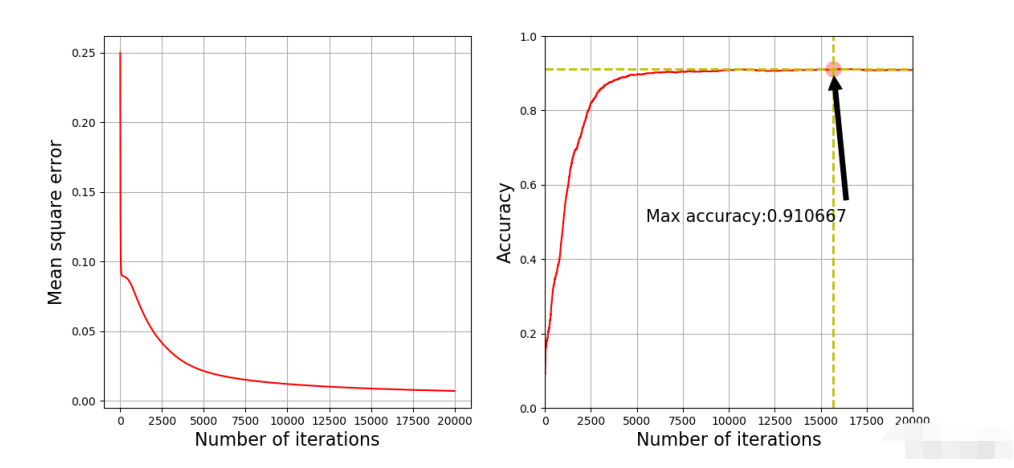
可以看出，模型只是跑通了，效果并不好，训练好几个小时准确率只有91%。原因可能是因为没有对模型进行正则化、学习率没有做动态调节等。

相反使用SVM模型准确率轻松可以达到97%以上。

# 获取数据
from sklearn.datasets import fetch_openml
from sklearn.svm import SVC
mnist = fetch_openml('mnist_784', version=1, as_frame=False) # 默认返回Pandas的DF类型
# sklearn加载的数据集类似字典结构
from sklearn.preprocessing import StandardScaler
X, y = mnist["data"], mnist["target"]
stder = StandardScaler() 
X = stder.fit_transform(X)
# 划分训练集与测试集
test_ratio = 0.3
 
shuffled_indices = np.random.permutation(X.shape[0]) # 打乱数据
test_set_size = int(X.shape[0] * test_ratio)
test_indices = shuffled_indices[:test_set_size]
train_indices = shuffled_indices[test_set_size:]
 
X_train, X_test, y_train, y_test = X[train_indices], X[test_indices], y[train_indices], y[test_indices]
# 训练SVM
 
cls_svm = SVC(C=1.0, kernel='rbf')
cls_svm.fit(X_train,y_train)
y_pre = cls_svm.predict(X_test)
acc_rate = np.sum(y_pre == y_test) / float(y_pre.shape[0])
acc_rate

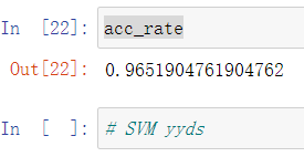
瑟瑟发抖~~~

最后将全部代码贴上：

import numpy as np
import matplotlib.pyplot as plt
import pickle
 
# 读取图片数据
def loadImageData(trainingDirName='data/', test_ratio=0.3):
    from os import listdir
    data = np.empty(shape=(0, 784))
    labels = np.empty(shape=(0, 1))
 
    for num in range(10):
        dirName = trainingDirName + '%s/' % (num)  # 获取当前数字文件路径
        # print(listdir(dirName))
        nowNumList = [i for i in listdir(dirName) if i[-3:] == 'bmp']  # 获取里面的图片文件
        labels = np.append(labels, np.full(shape=(len(nowNumList), 1), fill_value=num), axis=0)  # 将图片标签加入
        for aNumDir in nowNumList:  # 将每一张图片读入
            imageDir = dirName + aNumDir  # 构造图片路径
            image = plt.imread(imageDir).reshape((1, 784))  # 读取图片数据
            data = np.append(data, image, axis=0)  
    # 划分数据集
    m = data.shape[0]
    shuffled_indices = np.random.permutation(m)  # 打乱数据
    test_set_size = int(m * test_ratio)
    test_indices = shuffled_indices[:test_set_size]
    train_indices = shuffled_indices[test_set_size:]
 
    trainData = data[train_indices]
    trainLabels = labels[train_indices]
 
    testData = data[test_indices]
    testLabels = labels[test_indices]
 
    # 对训练样本和测试样本使用统一的均值 标准差进行归一化
    tmean = np.mean(trainData)
    tstd = np.std(testData)
 
    trainData = (trainData - tmean) / tstd
    testData = (testData - tmean) / tstd
    return trainData, trainLabels, testData, testLabels
 
# 对输出标签进行OneHot编码
def OneHotEncoder(labels,Label_class):
    one_hot_label = np.array([[int(i == int(labels[j])) for i in range(Label_class)] for j in range(len(labels))])
    return one_hot_label
 
# sigmoid激活函数
def sigmoid(z):
    for r in range(z.shape[0]):
        for c in range(z.shape[1]):
            if z[r,c] >= 0:
                z[r,c] = 1 / (1 + np.exp(-z[r,c]))
            else :
                z[r,c] = np.exp(z[r,c]) / (1 + np.exp(z[r,c]))
    return z
 
# 计算均方误差 参数：预测值 真实值
def cost(prediction, labels):
    return np.mean(np.power(prediction - labels,2))
 
 
# 训练一轮ANN 参数：训练数据 标签 输入层 隐层 输出层size 输入层隐层连接权重 隐层输出层连接权重 偏置1  偏置2 学习率
def trainANN(X, y, input_size, hidden_size, output_size, omega1, omega2, theta1, theta2, learningRate):
    # 获取样本个数
    m = X.shape[0]
    # 将矩阵X,y转换为numpy型矩阵
    X = np.matrix(X)
    y = np.matrix(y)
 
    # 前向传播 计算各层输出
    # 隐层输入 shape=m*hidden_size
    h_in = np.matmul(X, omega1.T) - theta1.T
    # 隐层输出 shape=m*hidden_size
    h_out = sigmoid(h_in)
    # 输出层的输入 shape=m*output_size
    o_in = np.matmul(h_out, omega2.T) - theta2.T
    # 输出层的输出 shape=m*output_size
    o_out = sigmoid(o_in)
 
    # 当前损失
    all_cost = cost(o_out, y)
 
    # 反向传播
    # 输出层参数更新
    d2 = np.multiply(np.multiply(o_out, (1 - o_out)), (y - o_out))
    omega2 += learningRate * np.matmul(d2.T, h_out) / m
    theta2 -= learningRate * np.sum(d2.T, axis=1) / m
 
    # 隐层参数更新
    d1 = np.multiply(h_out, (1 - h_out))
    omega1 += learningRate * (np.matmul(np.multiply(d1, np.matmul(d2, omega2)).T, X) / float(m))
    theta1 -= learningRate * (np.sum(np.multiply(d1, np.matmul(d2, omega2)).T, axis=1) / float(m))
 
    return omega1, omega2, theta1, theta2, all_cost
 
 
# 数据预测
def predictionANN(X, omega1, omega2, theta1, theta2):
    # 获取样本个数
    m = X.shape[0]
    # 将矩阵X,y转换为numpy型矩阵
    X = np.matrix(X)
 
    # 前向传播 计算各层输出
    # 隐层输入 shape=m*hidden_size
    h_in = np.matmul(X, omega1.T) - theta1.T
    # 隐层输出 shape=m*hidden_size
    h_out = sigmoid(h_in)
    # 输出层的输入 shape=m*output_size
    o_in = np.matmul(h_out, omega2.T) - theta2.T
    # 输出层的输出 shape=m*output_size
    o_out = np.argmax(sigmoid(o_in), axis=1)
 
    return o_out
 
 
# 计算模型准确率
def computeAcc(X, y, omega1, omega2, theta1, theta2):
    y_hat = predictionANN(X,omega1, omega2,theta1,theta2)
    return np.mean(y_hat == y)
 
 
if __name__ == '__main__':
    # 载入模型数据
    trainData, trainLabels, testData, testLabels = loadImageData()
 
    # 初始化设置
    input_size = 784
    hidden_size = 15
    output_size = 10
    lamda = 1
 
    # 将网络参数进行随机初始化
    omega1 = np.matrix((np.random.random(size=(hidden_size,input_size)) - 0.5) * 0.25) # 15*784
    omega2 = np.matrix((np.random.random(size=(output_size,hidden_size)) - 0.5) * 0.25)  # 10*15
 
    # 初始化两个偏置
    theta1 = np.matrix((np.random.random(size=(hidden_size,1)) - 0.5) * 0.25) # 15*1
    theta2 = np.matrix((np.random.random(size=(output_size,1)) - 0.5) * 0.25) # 10*1
    # 学习率
    learningRate = 0.1
    # 数据集
    m = trainData.shape[0] # 样本个数
    X = np.matrix(trainData) # 输入数据 m*784
    y_onehot=OneHotEncoder(trainLabels,10) # 标签 m*10
 
    iters_num = 20000  # 设定循环的次数
    loss_list = []
    acc_list = []
    acc_max = 0.0  # 最大精度 在精度达到最大时保存模型
    acc_max_iters = 0
 
    for i in range(iters_num):
        omega1, omega2, theta1, theta2, loss = trainANN(X, y_onehot, input_size, hidden_size, output_size, omega1,
                                                        omega2, theta1, theta2, learningRate)
        loss_list.append(loss)
        acc_now = computeAcc(testData, testLabels, omega1, omega2, theta1, theta2)  # 计算精度
        acc_list.append(acc_now)
        if acc_now > acc_max:  # 如果精度达到最大 保存模型
            acc_max = acc_now
            acc_max_iters = i  # 保存坐标 方便在图上标注
            # 保存模型参数
            f = open(r"./best_model", 'wb')
            pickle.dump((omega1, omega2, theta1, theta2), f, 0)
            f.close()
        if i % 100 == 0:  # 每训练100轮打印一次精度信息
            print("%d  Now accuracy : %f"%(i,acc_now))
 
    # 保存训练数据 方便分析
    f = open(r"./loss_list", 'wb')
    pickle.dump(loss_list, f, 0)
    f.close()
 
    f = open(r"./acc_list", 'wb')
    pickle.dump(loss_list, f, 0)
    f.close()
 
    # 绘制图形
    plt.figure(figsize=(13, 6))
    plt.subplot(121)
    x1 = np.arange(len(loss_list))
    plt.plot(x1, loss_list, "r")
    plt.xlabel(r"Number of iterations", fontsize=16)
    plt.ylabel(r"Mean square error", fontsize=16)
    plt.grid(True, which='both')
 
    plt.subplot(122)
    x2 = np.arange(len(acc_list))
    plt.plot(x2, acc_list, "r")
    plt.xlabel(r"Number of iterations", fontsize=16)
    plt.ylabel(r"Accuracy", fontsize=16)
    plt.grid(True, which='both')
    plt.annotate('Max accuracy:%f' % (acc_max),  # 标注最大精度值
                 xy=(acc_max_iters, acc_max),
                 xytext=(acc_max_iters * 0.7, 0.5),
                 arrowprops=dict(facecolor='black', shrink=0.05),
                 ha="center",
                 fontsize=15,
                 )
    plt.plot(np.linspace(acc_max_iters, acc_max_iters, 200), np.linspace(0, 1, 200), "y--", linewidth=2, )  # 最大精度迭代次数
    plt.plot(np.linspace(0, len(acc_list), 200), np.linspace(acc_max, acc_max, 200), "y--", linewidth=2)  # 最大精度
 
    plt.scatter(acc_max_iters, acc_max, s=180, facecolors='#FFAAAA')  # 标注最大精度点
    plt.axis([0, len(acc_list), 0, 1.0])  # 设置坐标范围
    plt.savefig("ANN_plot")  # 保存图片
    plt.show()

深度学习神经网络系列