Scipy简介_scipy的主要功能

Scipy简介

• Scipy依赖于Numpy
• Scipy包含的功能：最优化、线性代数、积分、插值、拟合、特殊函数、快速傅里叶变换、信号处理、图像处理、常微分方程求解器等
• 应用场景:Scipy是高端科学计算工具包，用于数学、科学、工程学等领域
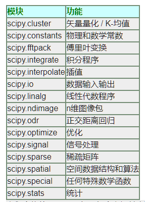
• Scipy由一些特定功能的子模块组成:
  

图片消噪处理

• scipy.fftpack模块用来计算快速傅里叶变换
  速度比传统傅里叶变换更快，是对之前算法的改进
  图片是二维数据，注意使用fftpack的二维转变方法

from scipy.fftpack import fft2, ifft2
import matplotlib.pyplot as plt
%matplotlib inline
import numpy as np
#读取照片数据
moon = plt.imread('moonlanding.png')	==>
array([[ 0.04705882,  0.        ,  0.23921569, ...,  0.        ,
         0.00392157,  0.53333336],
       [ 0.        ,  0.        ,  0.67843139, ...,  0.10196079,
         0.29019609,  0.        ],
       [ 0.72156864,  0.10980392,  0.60392159, ...,  0.        ,
         0.21568628,  1.        ],
       ..., 
       [ 0.00392157,  0.        ,  1.        , ...,  1.        ,
         1.        ,  0.95686275],
       [ 0.        ,  0.        ,  0.15686275, ...,  0.        ,
         0.        ,  0.35294119],
       [ 1.        ,  0.52156866,  0.04705882, ...,  0.        ,
         0.        ,  1.        ]], dtype=float32
#数据形式 
moon.shape		==> (474, 630)
#展示图片
plt.imshow(moon, cmap='gray')
#cmap 指定RGB的Z值，如果是三维数组则忽略cmap值
# 可选择的颜色映射参数为：Accent, Accent_r, Blues, Blues_r, BrBG, BrBG_r, BuGn, BuGn_r, BuPu, BuPu_r, CMRmap, CMRmap_r, Dark2, Dark2_r, GnBu, GnBu_r, Greens, Greens_r, Greys, Greys_r, OrRd, OrRd_r, Oranges, Oranges_r, PRGn, PRGn_r, Paired, Paired_r, Pastel1, Pastel1_r, Pastel2, Pastel2_r, PiYG, PiYG_r, PuBu, PuBuGn, PuBuGn_r, PuBu_r, PuOr, PuOr_r, PuRd, PuRd_r, Purples, Purples_r, RdBu, RdBu_r, RdGy, RdGy_r, RdPu, RdPu_r, RdYlBu, RdYlBu_r, RdYlGn, RdYlGn_r, Reds, Reds_r, Set1, Set1_r, Set2, Set2_r, Set3, Set3_r, Spectral, Spectral_r, Vega10, Vega10_r, Vega20, Vega20_r, Vega20b, Vega20b_r, Vega20c, Vega20c_r, Wistia, Wistia_r, YlGn, YlGnBu, YlGnBu_r, YlGn_r, YlOrBr, YlOrBr_r, YlOrRd, YlOrRd_r, afmhot, afmhot_r, autumn, autumn_r, binary, binary_r, bone, bone_r, brg, brg_r, bwr, bwr_r, cool, cool_r, coolwarm, coolwarm_r, copper, copper_r, cubehelix, cubehelix_r, flag, flag_r, gist_earth, gist_earth_r, gist_gray, gist_gray_r, gist_heat, gist_heat_r, gist_ncar, gist_ncar_r, gist_rainbow, gist_rainbow_r, gist_stern, gist_stern_r, gist_yarg, gist_yarg_r, gnuplot, gnuplot2, gnuplot2_r, gnuplot_r, gray, gray_r, hot, hot_r, hsv, hsv_r, inferno, inferno_r, jet, jet_r, magma, magma_r, nipy_spectral, nipy_spectral_r, ocean, ocean_r, pink, pink_r, plasma, plasma_r, prism, prism_r, rainbow, rainbow_r, seismic, seismic_r, spectral, spectral_r, spring, spring_r, summer, summer_r, tab10, tab10_r, tab20, tab20_r, tab20b, tab20b_r, tab20c, tab20c_r, terrain, terrain_r, viridis, viridis_r, winter, winter_r


# 傅里叶变换消噪

# 把时域空间转换到频域空间
f_moon = fft2(moon)

#关键步骤，过滤条件必须写好
# 在频域空间对高幅度的波进行过滤
f_moon[f_moon>3e2] = 0

# 把频域空间转回到时域空间
if_moon = np.real(ifft2(f_moon))

#展示
plt.imshow(if_moon, cmap="gray")

1
2
3
4
5
6
7
8
9
10
11
12
13
14
15
16
17
18
19
20
21
22
23
24
25
26
27
28
29
30
31
32
33
34
35
36
37
38
39
40
41
42

傅里叶级数转换介绍

• 图片灰度处理
  用二维数组展示的图片，没有RGB三原色，只有一个灰度值

# 利用数组随机数生成一个图片
data = np.random.randint(0,255,size=(1000,1000,3))

# astype 用来转换数组中数据的类型
plt.imshow(data.astype(np.uint8))
1
2
3
4
5

• jpg图像和png图像的区别
  • jpg图像 3个0-255之间的uint8类型整数来表示颜色
  • png图像 3个0-1之间的float32类型小数来表示颜色

back = plt.imread('back.jpg')
back.shape  ==>	(506, 900, 3)
back.dtype ==>dtype('uint8')
back.max(), back.min()  ==>(255, 0)
#取最大值或最小值
back.max(axis=2).shape 
plt.imshow(back.max(axis=2))
#取平均值
plt.imshow(back.mean(axis=2))
#用点乘积引入权重
weight = np.array([0.3,0.4,0.3])
plt.imshow(np.dot(back, weight), cmap="gray")

1
2
3
4
5
6
7
8
9
10
11
12
13

原照片

处理后

高数积分

• 使用 数值积分，求解圆周率

# 使用scipy.integrate进行积分，调用quad()方法
#定义圆函数
f = lambda x : (1-x**2)**0.5
#对积分区间切分
x = np.linspace(-1,1,100)
y = f(x)
#定义图像大小
plt.figure(figsize=(4,4))
#使图像横轴纵轴比例一致
plt.axis("equal")
#指定x、y的值域区间
plt.plot(x, y)
plt.plot(x, -y)

# 求不规则图形的面积
from scipy.integrate import quad
area, err = quad(f, a, b)	得到面积和误差==>
(1.5707963267948986, 1.0002356720661965e-09)
#用s/r^2得到圆周率
area*2/1**2		==>3.141592653589797

1
2
3
4
5
6
7
8
9
10
11
12
13
14
15
16
17
18
19
20
21

Scipy文件输入/输出

scipy.io

import scipy.io as io
1

随机生成数组，使用scipy中的io.savemat()保存
文件格式是.mat，标准的二进制文件

import scipy.io as scio

使用io.savemat()保存图片，数据必须用字典格式
#scio.savemat(file_name, mdict, appendmat=True, format='5', long_field_names=False, do_compression=False, oned_as='row')
scio.savemat('back.mat',{"data":back})

使用io.loadmat()读取数据
# scio.loadmat(file_name, mdict=None, appendmat=True, **kwargs)
scio.loadmat('back.mat')["data"]

#展示数据
plt.imshow(scio.loadmat('back.mat')["data"])
1
2
3
4
5
6
7
8
9
10
11
12

scipy.misc

• misc.imread()/imsave() 读写图片

from scipy import misc
#读取照片数据
#misc.imread(name, flatten=False, mode=None)
back = misc.imread('back.jpg')


#写入文件, misc.imsave(name, arr, format=None)
data = np.random.randint(0,255,size=(100,100,3))
# numpy series
data = data.astype(np.uint8)
misc.imsave('data.jpg', data)

#展示保存图片
plt.imshow(misc.imread('data.jpg'))
1
2
3
4
5
6
7
8
9
10
11
12
13
14

• misc的rotate、resize、imfilter操作

# 旋转图片
#1.读取照片数据（系统自带的照片），face = misc.face(gray=True)
face = misc.face(gray=True)
#2.展示 misc.imrotate(arr, angle, interp='bilinear')
plt.imshow(misc.imrotate(face, angle=70))



# 改变照片大小，misc.imresize(arr, size, interp='bilinear', mode=None)
#1.size使用0-1之间的小数，表示的是分数比
plt.imshow(misc.imresize(face, size=0.5))
#2.size使用整数，表示的是百分比
plt.imshow(misc.imresize(face, size=50))
#3.size使用元组，表示两个方向保留的像素点个数，取值是等间距取值
plt.imshow(misc.imresize(face, size=(30,60)))


#滤镜	Signature: misc.imfilter(arr, ftype)
# ftype的取值：'blur', 'contour', 'detail', 'edge_enhance', 'edge_enhance_more','emboss', 'find_edges', 'smooth', 'smooth_more', 'sharpen'.
plt.imshow(misc.imfilter(face, "emboss"),cmap="gray")

1
2
3
4
5
6
7
8
9
10
11
12
13
14
15
16
17
18
19
20
21

使用scipy.ndimage图片处理

使用scipy.misc.face(gray=True)获取图片，使用ndimage移动坐标、旋转图片、切割图片、缩放图片

from scipy import ndimage

# 1.shift移动坐标
'''
 ndimage.shift(input, shift, output=None, order=3, mode='constant', cval=0.0, prefilter=True)
mode(移动图片后空余部分的填充方式) 可选参数 'constant', 'nearest', 'reflect', 'mirror' or 'wrap'
shift 移动的范围，给定的数值是float则x,y移动相同距离，也可以给定一个列表

'''
plt.imshow(ndimage.shift(face,shift=200,mode="constant"), cmap="gray")
plt.imshow(ndimage.shift(face,shift=[100,100],mode="mirror"))


# rotate旋转图片
'''
ndimage.rotate(input, angle, axes=(1, 0), reshape=True, output=None, order=3, mode='constant', cval=0.0, prefilter=True)
'''
plt.imshow(ndimage.rotate(face, angle=60))

# zoom缩放图片
'''
 ndimage.zoom(input, zoom, output=None, order=3, mode='constant', cval=0.0, prefilter=True)
 zoom接受一个比例列表，表示不同的轴上的比值
'''
plt.imshow(ndimage.zoom(face,zoom=0.5))
plt.imshow(ndimage.zoom(face,zoom=[0.3,2]))

1
2
3
4
5
6
7
8
9
10
11
12
13
14
15
16
17
18
19
20
21
22
23
24
25
26
27

• 图片进行过滤
  添加噪声，对噪声图片使用ndimage中的高斯滤波、中值滤波、signal中维纳滤波进行处理
  使图片变清楚

# 加载图片，使用灰色图片misc.face()添加噪声
moon = plt.imread('moonlanding.png')
plt.imshow(moon, cmap="gray")

#gaussian高斯滤波参数sigma：高斯核的标准偏差
'''
ndimage.gaussian_filter(input, sigma, order=0, output=None, mode='reflect', cval=0.0, truncate=4.0)
'''
plt.imshow(ndimage.gaussian_filter(moon, sigma=0.8), cmap="gray")


#median中值滤波
'''
ndimage.median_filter(input, size=None, footprint=None, output=None, mode='reflect', cval=0.0, origin=0)
参数size：给出在每个元素上从输入数组中取出的形状位置，定义过滤器功能的输入
'''
plt.imshow(ndimage.median_filter(moon, size=6), cmap="gray")


#signal维纳滤波
'''
signal.wiener(im, mysize=None, noise=None)
参数mysize：滤镜尺寸的标量
'''
import scipy.signal as signal
plt.imshow(signal.wiener(moon, mysize=6), cmap="gray")

1
2
3
4
5
6
7
8
9
10
11
12
13
14
15
16
17
18
19
20
21
22
23
24
25
26
27

pandas绘图函数

Series和DataFrame都有一个用于生成各类图表的plot方法。默认情况下，它们所生成的是线形图

• matplotlib来绘制
• 格式： s.plot(kind=‘line’, ax=None, figsize=None, use_index=True, title=None, grid=None, legend=False, style=None, logx=False, logy=False, loglog=False, xticks=None, yticks=None, xlim=None, ylim=None, rot=None, fontsize=None, colormap=None, table=False, yerr=None, xerr=None, label=None, secondary_y=False, **kwds)
  • 参数kind用来指定绘制图像类型：
    • ‘line’ : line plot (default)
    • ‘bar’ : vertical bar plot
    • ‘barh’ : horizontal bar plot
    • ‘hist’ : histogram
    • ‘box’ : boxplot
    • ‘kde’ : Kernel Density Estimation plot
    • ‘density’ : same as ‘kde’
    • ‘area’ : area plot
    • ‘pie’ : pie plot

# pandas整合的一些图形的绘制办法
# 绘图要先导入包
import numpy as np
import pandas as pd
from pandas import Series,DataFrame
import matplotlib.pyplot as plt
# 在当前文本编辑器中绘制图像
%matplotlib inline
1
2
3
4
5
6
7
8

线形图line

• 一般用于描述数据变化趋势
• 线型图最常用的横坐标就是时间

# data是要展示的数据
data = np.random.randint(0,100,size=(10))
# 横坐标
x = np.arange(10)
# Series绘制的线性图是单条线， index作为横坐标， values作为展示的数据
s = Series(data=data, index=x)
s.plot(kind="line")		==>图一


# DataFrame绘制多条线，每一列作为一条线绘制
df  ==>
	A	B
0	76	51
1	93	36
2	88	59
3	55	75
4	11	9
5	43	35
6	10	67
7	43	51
8	54	42
9	39	74
df.plot(kind="line")	==> 图二

1
2
3
4
5
6
7
8
9
10
11
12
13
14
15
16
17
18
19
20
21
22
23
24

图一

图二

柱状图bar

Series柱状图示例,kind = ‘bar’/‘barh’

• 一般用于数据间的横向比较

# 1.Series 数据
data = [10,16,19,18]
# 默认不支持汉语显示
x = ["tom","jack","lucy","mery"]
s = Series(data=data, index=x)
s.plot(kind="bar")
# 2.DataFrame数据
df = DataFrame({
    "python":[89,78,99],
    "C":[70,75,80],
    "PHP":[11,15,10]
}, index=["tom","lucy","jack"])
df.plot(kind="bar")
1
2
3
4
5
6
7
8
9
10
11
12
13

Series

DataFrame

直方图hist

• 直方图是用来表示频率的图像
  • 每一个柱子的高度，表示的是在该数据区间，数据出现的次数。 每一个柱子的宽度，表示的是数据区间，默认是10个柱子，把数据从最大值~最小值平均分成10个区间
  • 参数bins可以设置直方图方柱的个数上限，越大柱宽越小，数据分组越细致
  • 设置normed参数为True，可以把频数转换为概率
  • kde图：核密度估计，用于弥补直方图由于参数bins设置的不合理导致的精度缺失问题

s = Series(data=np.random.randn(100))
# bins可能会导致直方图绘制不合理，所以一般会结合kde一起展示，但是要使用normed统一单位
# normed=True，柱高表示该区间数据出现的概率
s.plot(kind="hist", bins=8, normed=True)
s.plot(kind="kde")

1
2
3
4
5
6

散点图scatter

• 散布图 散布图是观察两个一维数据数列之间的关系的有效方法,DataFrame对象可用
• 使用方法： 设置kind = ‘scatter’，给明标签columns

df = DataFrame(data={
    "X":[1,3,5,7,9],
    "Y":[3,6,8,9,0],
    "M":[10,10,12,8,11],
})

# dataFrame对象绘制散点图与索引无关，一般就是查看某两列数据之间的对应关系
df.plot(kind="scatter",x="Y",y="M")

1
2
3
4
5
6
7
8
9

• 散布图矩阵，当有多个点时，两两点的关系

  • 使用函数：pd.plotting.scatter_matrix(),

    pd.plotting.scatter_matrix(frame, alpha=0.5, figsize=None, ax=None, grid=False, diagonal=‘hist’, marker=’.’, density_kwds=None, hist_kwds=None, range_padding=0.05, **kwds)

  • 参数diagnol：设置对角线的图像类型

pd.plotting.scatter_matrix(df,diagonal="hist")
1