
- 1Postman打不开/黄屏/一直转圈/Windows_postman安装以后加载不出来
- 2Linux下rabbitmq运维相关:日志、自定义配置等_rabbitmq日志 超过8g
- 3【监控系统】日志可视化监控体系ELK搭建_elk日志监控平台
- 4博士申请 | 新加坡国立大学Robby T. Tan教授招收计算机视觉方向博士生
- 5Python - 深夜数据结构与算法之 BFS & DFS_python的bfs\dfs算法
- 6探索未来:Java在人工智能领域的崛起_人工智能在java后端开发中应用与挑战文章
- 7用Python实现OpenCV特征提取与图像检索 | Demo
- 8搭建 Kafka 前需要考虑什么方面?_算kafka资源时,需要考虑的因素有
- 95款开源BI系统倾力推荐,企业信息化的利器_国内开源的bi系统
- 10Github如何下载单个文件夹_github下载单个文件夹
CV领域Transformer这一篇就够了(原理详解+pytorch代码复现)_transformer卷积实现
赞
踩
这一篇不够不够,当时年轻瞎写的,臭长的文章懒得改了,看别的博客吧 (˚ ˃̣̣̥᷄⌓˂̣̣̥᷅ ) 。
前言
本文主要介绍:注意力机制、自注意力机制、多头注意力机制、ViT、Swin Tranformer、其他Transformer的改进,并配合代码实现。
参考链接:
(饭范仁义-AI编程)https://www.bilibili.com/video/BV1nL4y1j7hA?spm_id_from=333.999.0.0&vd_source=b2549fdee562c700f2b1f3f49065201b
(霹雳巴啦Wz)https://blog.csdn.net/qq_37541097/article/details/117691873
一、注意力机制
1.1注意力机制通俗理解
注意力机制本质上与人类对外界事物的观察机制相似。通常来说,人们在观察外界事物的时候,首先会比较关注比较倾向于观察事物某些重要的局部信息,然后再把不同区域的信息组合起来,从而形成一个对被观察事物的整体印象,实现关注重要有用信息,抑制其他无用信息。
Attention机制最先应用在自然语言处理方面,主要是为了改进文本之间的编码方式,通过编码-解码之后能学习到更好的序列信息。
可以总体上分为两类:
聚焦式(focus)注意力:自上而下的有意识的注意力,主动注意——是指有预定目的、依赖任务的、主动有意识地聚焦于某一对象的注意力;
显著性(saliency-based)注意力:自下而上的有意识的注意力,被动注意——基于显著性的注意力是由外界刺激驱动的注意,不需要主动干预,也和任务无关;可以将max-pooling和门控(gating)机制来近似地看作是自下而上的基于显著性的注意力机制。
在人工神经网络中,注意力机制一般就特指聚焦式注意力。
1.2注意力机制计算公式
现在你可能还看不懂这个公式具体在讲什么,接下来我将详细简明的阐述。
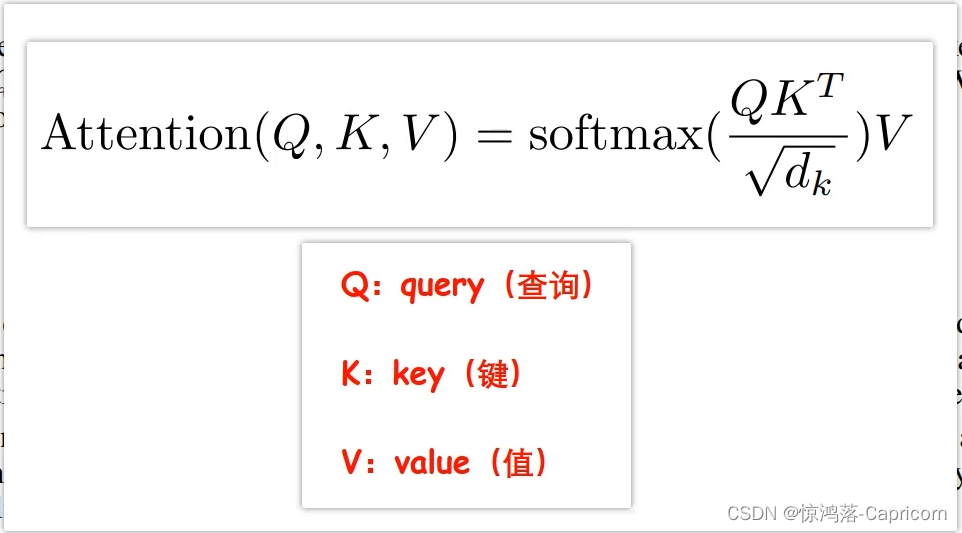
第一阶段,需要三个指定的输入Q(query),K(key),V(value),可以引入不同函数和计算机制,根据Q和K,计算两者的相似性和相关性,d为K的维度dim。
第二阶段,引入类似的softmax的计算方式对第一阶段得分进行数值转换,一方面可以进行归一化,计算所有元素权重之和为1,另一方面可以通过softmax突出元素的权重。
第三阶段,通过计算结果a和V对应的权重系数,然后加权求和得到Attention数值。
(当输入的Q=K=V时,称作自注意力计算规则)。
举个例子:

Q(查询)和K(键)转置进行点乘(对于位置相乘求和),得到了各项查询的相似度,再除d,得到的是一个实数值,使用softmax将其变为权重(小于1的值),相似度权重x价值,就是求得的注意力。
1.3注意力机制计算过程
1.Input:输入Q、K、V三个向量;
2.a(i,j):每个qi分别和不同的kj乘,得a(i,j) = qi · kj;(应该是K的转置),a(i,j)为一个实数值。
3.除dim:为了梯度的稳定,Transformer使用了归一化,对a(i,j) 除以根号d,(d为k的维度);
4.softmax:对同一个i的a(i,j) ,施以softmax激活函数;
5.乘V:对于每个i,a(i,j)乘vj后求和,得到加权的每个输入向量ai的注意力评分bi;
q:代表query,后续会去和每一个k进行匹配(相乘)
k:代表key,后续会被每个q匹配(相乘)
v:代表从a 中提取得到的信息
后续q 和k 匹配的过程可以理解成计算两者的相关性,相关性越大对应v 的权重也就越大。
通过上述讲解,我们了解了单个qi是如何求注意力评分bi的,接下来仅需合并成矩阵,进行并行运算,一次求得多个输入的注意力评分矩阵B。

1.Q和K转置进行点乘,除根号d,进softmax,得相关性矩阵
2.相关性矩阵乘V得注意力评分矩阵B
Attention机制的实质其实就是一个寻址(addressing)的过程,如上图所示:给定一个和任务相关的查询Query向量 q,通过计算与Key的注意力分布并附加在Value上,从而计算Attention Value,这个过程实际上是Attention机制缓解神经网络模型复杂度的体现:不需要将所有的N个输入信息都输入到神经网络进行计算,只需要从中选择一些和查询Query相关的信息输入给神经网络。
1.4注意力机制代码
# pytorch实现
import torch
import torch.nn as nn
import torch.nn.functional as F

# 缩放点积注意力
class ScaledDotProductAttention(nn.Module):
    ''' Scaled Dot-Product Attention '''

    def __init__(self, temperature, attn_dropout=0.1):
        super().__init__()
        # temperature是k的维度dk
        self.temperature = temperature
        self.dropout = nn.Dropout(attn_dropout)

	#外部输入q、k、v
    def forward(self, q, k, v, mask=None):
        # a = (q/dk) 与 k的转置 矩阵相乘
        attn = torch.matmul(q / self.temperature, k.transpose(2, 3))

        # 是否进行mask
        if mask is not None:
            attn = attn.masked_fill(mask == 0, -1e9)

        # softmax+dropout得到相似性矩阵
        attn = self.dropout(F.softmax(attn, dim=-1))
        # 相似性矩阵与v矩阵相乘,得注意力评价矩阵
        output = torch.matmul(attn, v)

        # 返回:注意力评价矩阵 和 相似性矩阵
        return output, attn
- 1
- 2
- 3
- 4
- 5
- 6
- 7
- 8
- 9
- 10
- 11
- 12
- 13
- 14
- 15
- 16
- 17
- 18
- 19
- 20
- 21
- 22
- 23
- 24
- 25
- 26
- 27
- 28
- 29
- 30
- 31
- 32
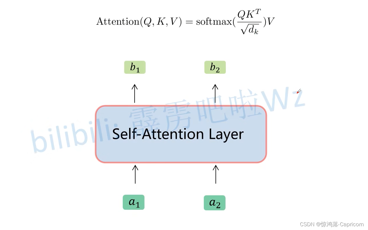
二、自注意力机制
2.1 注意力机制和自注意力机制的区别
自注意力机制:Query=Key=Value=输入
传统的Attention:
Q来自于外部,K、V
Q在Decoder目标处,K、V在Encoder源头处self-Attention:
Q、K、V是对自身(self)输入的变换
Q、K、V在同一处(Decoder目标或Encoder源头处)
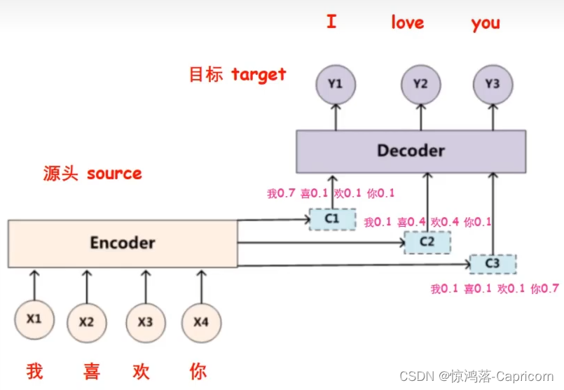
2.2 编码-译码中的attention
汉译英编码-译码模型:
无attention的编码-译码模型

有attention的编码-译码模型
2.3自注意力机制计算流程
1.Input:输入单词或图片xi;
2.Embedding:将单词、图片转化为转化成嵌入向量ai;
3.Querys、Keys、Values:a分别对Wq、Wk、Wv(这三个参数是可训练的,是共享的)矩阵乘法,得到Q、K、V三个向量;
4.a(i,j):每个qi分别和不同的kj乘,得a(i,j) = qi · kj;(应该是K的转置),a(i,j)为一个实数值。
5.除dim:为了梯度的稳定,Transformer使用了归一化,对a(i,j) 除以根号d,(d为k的维度);
6.softmax:对同一个i的a(i,j) ,施以softmax激活函数;
7.乘V:对于每个i,a(i,j)乘vj后求和,得到加权的每个输入向量ai的注意力评分bi;


矩阵计算:
1.X进行Embeding后得到输入矩阵A
2.A分别与Wq、Wk、Wv相乘得到Q、K、V矩阵
3.Q和K转置进行点乘,除根号d,进softmax,得相关性矩阵
4.相关性矩阵乘V得注意力评分矩阵B
self-attention就是对输入向量的权重进行调整。
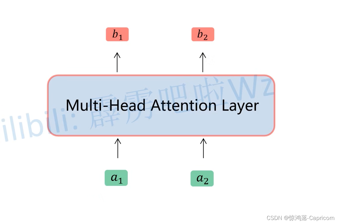
三、多头注意力机制
刚刚已经聊完了Self-Attention模块,接下来再来看看Multi-Head Attention模块,实际使用中基本使用的还是Multi-Head Attention模块。其实只要懂了Self-Attention模块Multi-Head Attention模块就非常简单了,多头注意力就是对单头注意力的简单堆叠。
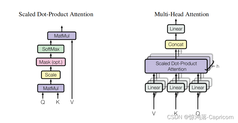
3.1多头注意力机制计算过程
(无embeding操作)
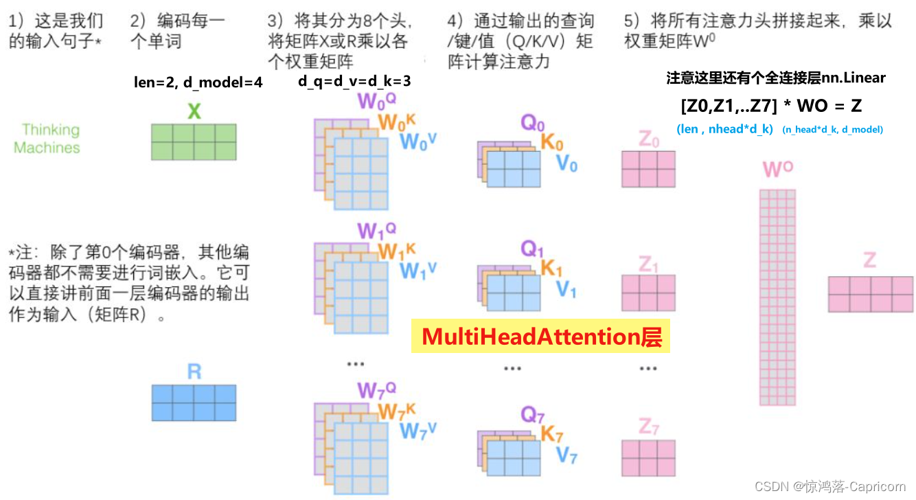
就是和attention类似,将输入X分别通过多组不同的Wqi、Wki、Wvi得到多组不同的Qi、Ki、Vi,然后得到了不同的结果,进行拼接,通过线性层乘Wo得到与输入矩阵维度相等的结果。


3.2 多头自注意力机制计算过程
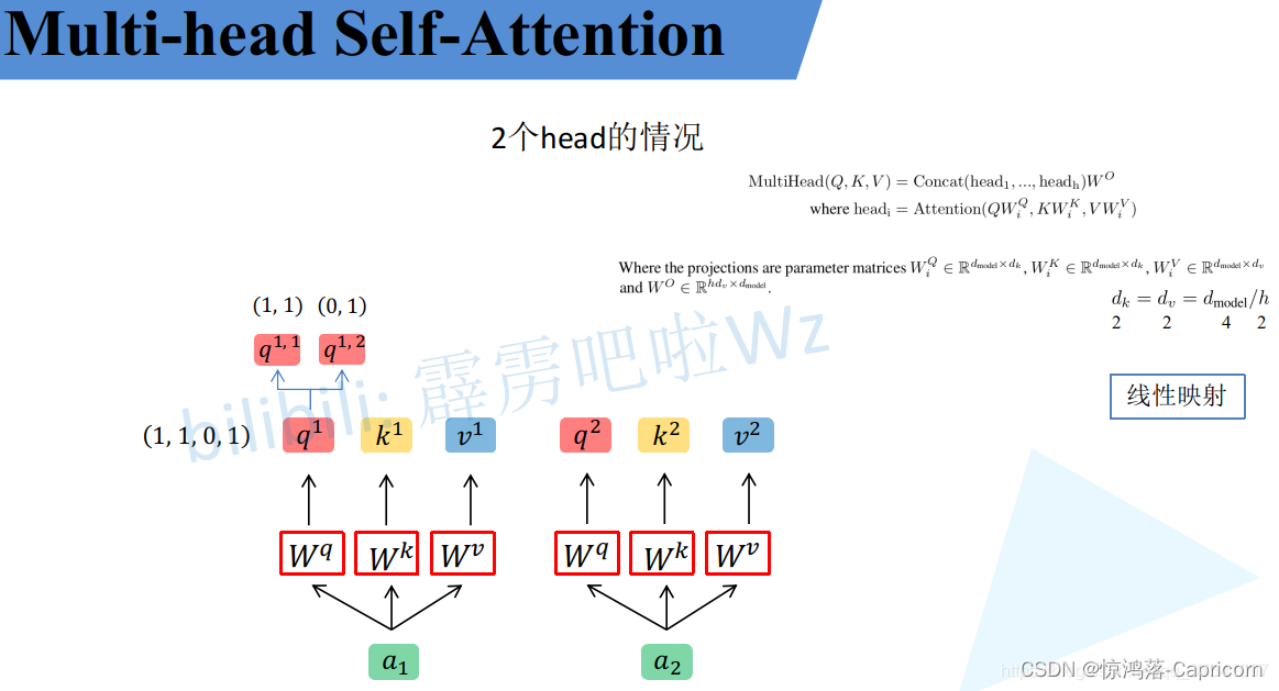
1.QKV分头:
对得到的qi、ki、vi按n个head(n=2)进行均分为q(i,j)、k(i,j)、v(i,j),(其中j=1~n)
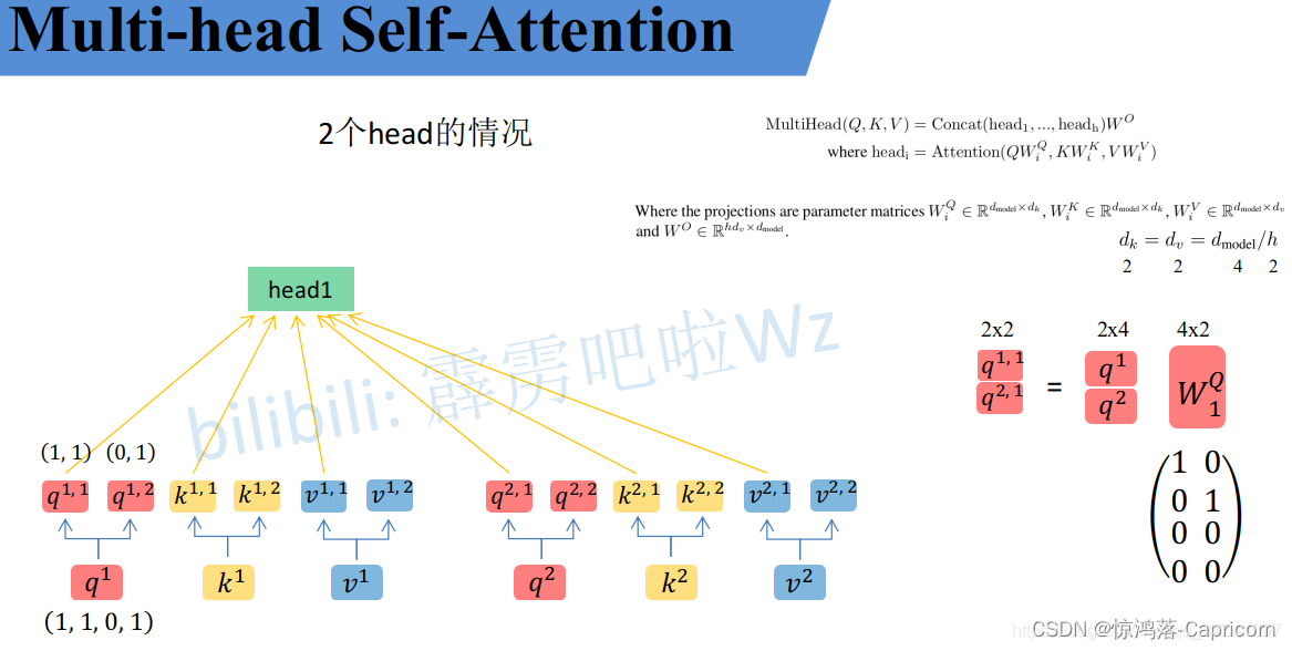
2.对于每个 j 的q、k、v 是一个头,共分为n个头,如上图的q(i,1)、k(i,1)、v(i,1)是一个head(i=1和2)

3.对每个head,执行self-attention的同样的操作,对每组q(i,j)、k(i,j)、v(i,j)求得 自注意力评分b(i,j).

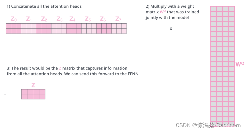
4. b(i,j)按照二维矩阵 拼接成B,B乘以Wo。( Wo的作用:是保证multi-head-self-attention输出的向量和输入的长度一致。)

Multi-head-self-attention最终效果:
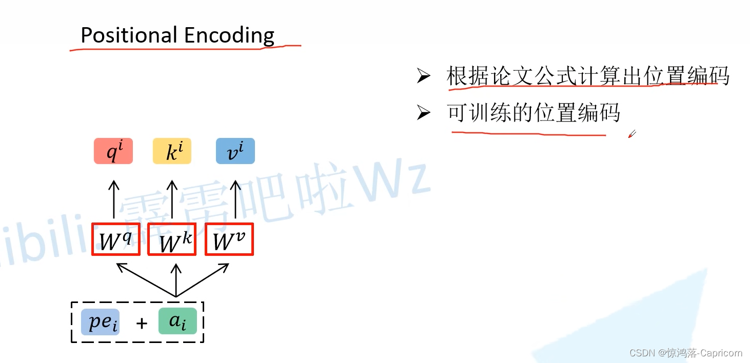
3.3位置编码
位置编码要和ai相加,则shape的ai一样。

四、Vision Teansformer(ViT)

ViT由3个模块组成:
Linear Projection of Flattened Patches(Embedding层):Patch embedding+Position embedding+Class token输入Encoder层
Transformer Encoder(Encoder层):将上图右边的结构重复堆叠L次
MLP Head(最终用于分类的层结构):只提取Class token的输出,进行得到分类的结果
4.1 Embedding层
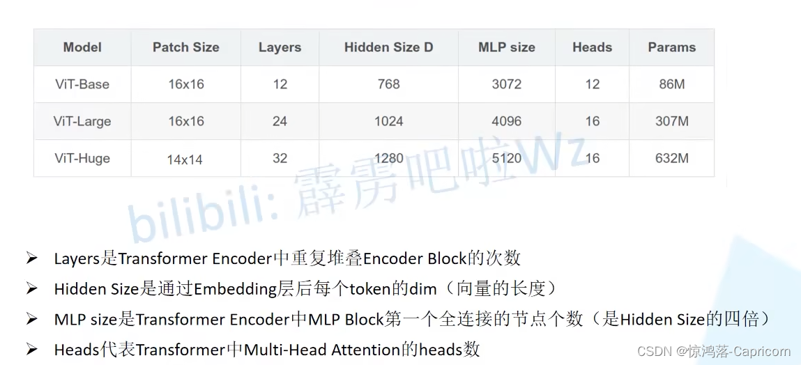
对于标准的Transformer模块,要求输入的是token(向量)序列,即二维矩阵[num_token, token_dim],如下图,token0-token9对应的都是向量,以ViT-B/16为例,每个token向量长度为768。
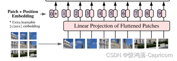
对于图像数据而言,其数据格式为 [H, W, C] 是三维矩阵明显不是Transformer想要的。所以需要先通过一个Embedding层来对三维数据变换为二维数据。如下图所示,首先将一张图片按给定大小分成一堆Patches(图片块)。
以ViT-B/16为例,将大小224x224的输入图片按照16x16大小的Patch进行划分,划分后会得到196个Patches。接着通过线性映射将每个Patch映射到一维向量中,每个Patche数据shape为[16, 16, 3]通过映射得到一个长度为768的token向量(后面都直接称为token)。[16, 16, 3] -> [768]
在代码实现中,直接通过一个卷积层来实现。 以ViT-B/16为例,直接使用一个卷积核大小为16x16,stride为16,卷积核个数为768的卷积来实现。通过卷积[224, 224, 3] -> [14, 14, 768],然后把H以及W两个维度展平[W,H,C]->[W*H,C],如[14, 14, 768] -> [196, 768],此时正好变成了一个二维矩阵,正是Transformer想要的。
在输入Transformer Encoder之前注意需要加上图片类别 [class]token 放在positoin=0处以及叠加Position Embedding。 以ViT-B/16为例,就是一个长度为768的向量,与之前从图片中生成的tokens拼接在一起,Cat([1, 768], [196, 768]) -> [197, 768]。然后关于Position Embedding就是之前Transformer中讲到的Positional Encoding,这里的Position Embedding采用的是一个可训练的参数是直接叠加在tokens上的(add),所以shape要一样。以ViT-B/16为例,刚刚拼接[class]token后shape是[197, 768],那么这里的Position Embedding的shape也是[197, 768]。对于Position Embedding作者也有做一系列对比试验,在源码中默认使用的是1D Pos. Emb。

图片中每个patch求得的token 都有一个位置编码,这些位置编码彼此间的余弦相似度如上图。黄色相似度高,蓝色相似度低。亮点就是对应该token的位置编码在原图中的位置。这就是最终学习到的位置编码。
4.2 Encoder层
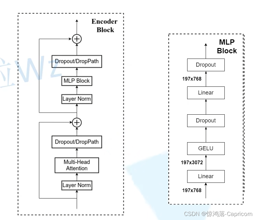
Transformer Encoder其实就是堆叠Encoder Block重复 L次,Encoder Block,主要由以下几部分组成:
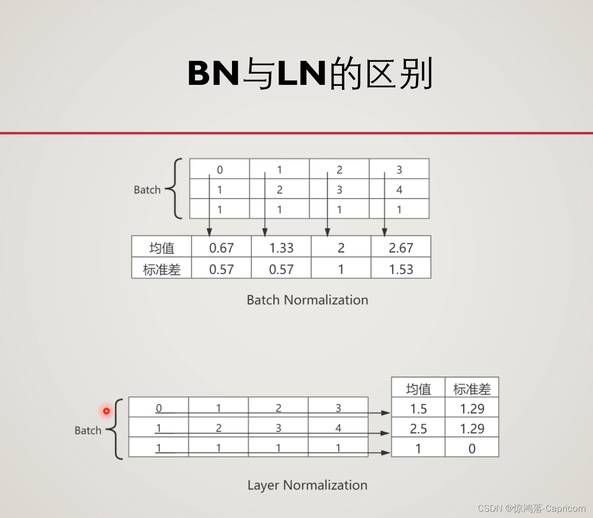
·Layer Norm,这种Normalization方法主要是针对NLP领域提出的,这里是对每个token进行Norm处理。

·Multi-Head Attention,这个结构之前在讲Transformer中很详细的讲过,不再赘述。
·Dropout/DropPath,在原论文的代码中是直接使用的Dropout层,在但实现代码中使用的是DropPath(stochastic depth),可能后者会更好一点。(不了解Droppath的可以看这篇介绍Droppath通俗易懂)
·MLP Block,如上图右侧所示,就是全连接+GELU激活函数+Dropout组成也非常简单,需要注意的是第一个全连接层会把输入节点个数翻4倍[197, 768] -> [197, 3072],第二个全连接层会还原回原节点个数[197, 3072] -> [197, 768]
·残差结构, 将输入与dropout层输出相加。
4.3 MLP Head层
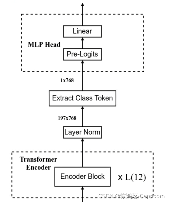
其中pre-logits就是一个全连接层+tanh激活函数。
下图是ViT-B/16的一个总体结构:

4.4 ViT代码实现
"""
original code from rwightman:
https://github.com/rwightman/pytorch-image-models/blob/master/timm/models/vision_transformer.py
"""
from functools import partial
from collections import OrderedDict

import torch
import torch.nn as nn


def drop_path(x, drop_prob: float = 0., training: bool = False):
    if drop_prob == 0. or not training:
        return x
    keep_prob = 1 - drop_prob
    shape = (x.shape[0],) + (1,) * (x.ndim - 1)  # work with diff dim tensors, not just 2D ConvNets
    random_tensor = keep_prob + torch.rand(shape, dtype=x.dtype, device=x.device)
    random_tensor.floor_()  # binarize
    output = x.div(keep_prob) * random_tensor
    return output


class DropPath(nn.Module):
    """
    Drop paths (Stochastic Depth) per sample  (when applied in main path of residual blocks).
    """
    def __init__(self, drop_prob=None):
        super(DropPath, self).__init__()
        self.drop_prob = drop_prob

    def forward(self, x):
        return drop_path(x, self.drop_prob, self.training)


# PatchEmbedding层(通过卷积实现)
class PatchEmbed(nn.Module):
    """
    2D Image to Patch Embedding
    """
    def __init__(self, img_size=224, patch_size=16, in_c=3, embed_dim=768, norm_layer=None):
        super().__init__()
        img_size = (img_size, img_size)  # img_size图片大小
        patch_size = (patch_size, patch_size)  # patch_size图像块大小(也是卷积核大小)
        self.img_size = img_size
        self.patch_size = patch_size
        self.grid_size = (img_size[0] // patch_size[0], img_size[1] // patch_size[1])  # //表取整除
        self.num_patches = self.grid_size[0] * self.grid_size[1]

        # 定义卷积层proj,in_c输入通道数(rgb3通道),embed_dim卷积核个数(卷积层输出通道数)
        self.proj = nn.Conv2d(in_c, embed_dim, kernel_size=patch_size, stride=patch_size)
        # 如果norm_layer不为空,则进行正则化,
        self.norm = norm_layer(embed_dim) if norm_layer else nn.Identity()

    def forward(self, x):
        # 输入图像X
        # assert检查输入图像大小,B(batch_size), C(channel), H(height), W(weight)
        B, C, H, W = x.shape
        assert H == self.img_size[0] and W == self.img_size[1], \
            f"Input image size ({H}*{W}) doesn't match model ({self.img_size[0]}*{self.img_size[1]})."

        # proj(卷积)
        # flatten(压平H,W): [B, C, H, W] -> [B, C, HW]
        # transpose(交换后两维): [B, C, HW] -> [B, HW, C]
        x = self.proj(x).flatten(2).transpose(1, 2)
        x = self.norm(x)
        return x


# Encoder Block中的MultiHead-Self-Attention层
class Attention(nn.Module):
    def __init__(self,
                 dim,   # 输入token的dim
                 num_heads=8,  # head数
                 qkv_bias=False,  # 生成qkv不用bais
                 qk_scale=None,  # None时使用:根号dk分之一
                 attn_drop_ratio=0.,  # dropout率
                 proj_drop_ratio=0.):  # dropout率
        super(Attention, self).__init__()
        self.num_heads = num_heads
        head_dim = dim // num_heads  # 分头:计算每个head均分得到的q,k,v个数
        self.scale = qk_scale or head_dim ** -0.5  # qk_scale是根号下head_dim分之一,就是q*k转置后乘的那个:根号dk分之一
        self.qkv = nn.Linear(dim, dim * 3, bias=qkv_bias)  # 通过qkv全连接层:(q,k,v)=X·(Wq,Wk,Wv),一次并行求得qkv
        # 全连接层:in_features输入特征个数=dim,out_features输出特征个数(全连接层节点个数)=dim*3
        self.attn_drop = nn.Dropout(attn_drop_ratio)
        self.proj = nn.Linear(dim, dim)  # 通过proj全连接层:B=B·Wo,进行bij->bi拼接后的映射
        self.proj_drop = nn.Dropout(proj_drop_ratio)

    def forward(self, x):
        # [batch_size, num_patches + 1, total_embed_dim]
        # (num_patches + 1的1是class token,num_patches + 1个向量大小都是total_embed_dim)
        B, N, C = x.shape

        # qkv(): -> [batch_size, num_patches + 1, 3 * total_embed_dim]
        # reshape分qkv分头: -> [batch_size, num_patches + 1, 3, num_heads, embed_dim_per_head]
        # permute调序: -> [3, batch_size, num_heads, num_patches + 1, embed_dim_per_head]
        qkv = self.qkv(x).reshape(B, N, 3, self.num_heads, C // self.num_heads).permute(2, 0, 3, 1, 4)
        # 切片q、k、v,都是[batch_size, num_heads, num_patches + 1, embed_dim_per_head]
        q, k, v = qkv[0], qkv[1], qkv[2]  # make torchscript happy (cannot use tensor as tuple)

        # transpose:原q、k、v-> [batch_size, num_heads, embed_dim_per_head, num_patches + 1]
        # @ 矩阵乘法: 多维矩阵乘法只乘最后两维 -> [batch_size, num_heads, num_patches + 1, num_patches + 1]
        # q乘k转置,乘根号dk
        attn = (q @ k.transpose(-2, -1)) * self.scale
        # dim=-1表示attn在每一行进行softmax处理
        attn = attn.softmax(dim=-1)
        attn = self.attn_drop(attn)

        # @ 矩阵乘法: -> [batch_size, num_heads, num_patches + 1, embed_dim_per_head]
        # transpose: -> [batch_size, num_patches + 1, num_heads, embed_dim_per_head]
        # reshape: -> [batch_size, num_patches + 1, total_embed_dim]
        # softmax(qk相似度) 乘 v,reshape进行bij->bi的拼接映射
        x = (attn @ v).transpose(1, 2).reshape(B, N, C)
        # 通过proj全连接层:B=B·Wo映射
        x = self.proj(x)
        x = self.proj_drop(x)
        return x


# Encoder Block中的MLP(两个全连接层)
class Mlp(nn.Module):
    """
    MLP as used in Vision Transformer, MLP-Mixer and related networks
    """
    # in_features输入特征个数,hidden_features第一个全连接层节点个数,out_features第二个全连接层节点个数,act_layer激活函数
    def __init__(self, in_features, hidden_features=None, out_features=None, act_layer=nn.GELU, drop=0.):
        super().__init__()
        out_features = out_features or in_features  # out_features=None,in_features
        hidden_features = hidden_features or in_features  # 同上
        self.fc1 = nn.Linear(in_features, hidden_features)
        self.act = act_layer()  # GELU激活函数
        self.fc2 = nn.Linear(hidden_features, out_features)
        self.drop = nn.Dropout(drop)

    def forward(self, x):
        x = self.fc1(x)
        x = self.act(x)
        x = self.drop(x)
        x = self.fc2(x)
        x = self.drop(x)
        return x


# Encoder Block
class Block(nn.Module):
    def __init__(self,
                 dim,  # token 的dim
                 num_heads,  # head数
                 mlp_ratio=4.,  # mlp中第一个全连接层的节点个数是输入的4倍
                 qkv_bias=False,  # 是否使用bias
                 qk_scale=None,  # 根号dk分之一
                 drop_ratio=0.,  # attention中的drop_out率
                 attn_drop_ratio=0.,  # attention中的drop_out率
                 drop_path_ratio=0.,  # Encoder Block中的drop_path率
                 act_layer=nn.GELU,  # 激活函数
                 norm_layer=nn.LayerNorm):  # normalization使用LayerNorm

        super(Block, self).__init__()
        # 实例化LayerNorm层
        self.norm1 = norm_layer(dim)
        # 实例化Attention层
        self.attn = Attention(dim, num_heads=num_heads, qkv_bias=qkv_bias, qk_scale=qk_scale, attn_drop_ratio=attn_drop_ratio, proj_drop_ratio=drop_ratio)
        # NOTE: drop path for stochastic depth, we shall see if this is better than dropout here
        # 实例化DropPath层
        self.drop_path = DropPath(drop_path_ratio) if drop_path_ratio > 0. else nn.Identity()

        # 实例化LayerNorm层
        self.norm2 = norm_layer(dim)
        mlp_hidden_dim = int(dim * mlp_ratio)
        # 实例化Mlp层
        self.mlp = Mlp(in_features=dim, hidden_features=mlp_hidden_dim, act_layer=act_layer, drop=drop_ratio)

    def forward(self, x):
        # 这里的+=都引入了恒等映射的残差思想
        x = x + self.drop_path(self.attn(self.norm1(x)))
        x = x + self.drop_path(self.mlp(self.norm2(x)))
        return x


# ViT
class VisionTransformer(nn.Module):
    def __init__(self, img_size=224, patch_size=16, in_c=3, num_classes=1000,
                 embed_dim=768, depth=12, num_heads=12, mlp_ratio=4.0, qkv_bias=True,
                 qk_scale=None, representation_size=None, distilled=False, drop_ratio=0.,
                 attn_drop_ratio=0., drop_path_ratio=0., embed_layer=PatchEmbed, norm_layer=None,
                 act_layer=None):
        """
        Args:
            img_size (int, tuple): input image size
            patch_size (int, tuple): patch size
            in_c (int): number of input channels
            num_classes (int): number of classes for classification head
            embed_dim (int): embedding dimension,patch embedding层卷积核个数
            depth (int): 是Encoder重复次数,depth of transformer
            num_heads (int): number of attention heads
            mlp_ratio (int): ratio of mlp hidden dim to embedding dim
            qkv_bias (bool): enable bias for qkv if True
            qk_scale (float): override default qk scale of head_dim ** -0.5 if set
            representation_size (Optional[int]):是否构建MLP层的pre-logits,enable and set representation layer (pre-logits) to this value if set
            distilled (bool): 为了兼容搭建DeiT的参数,model includes a distillation token and head as in DeiT models
            drop_ratio (float): dropout rate
            attn_drop_ratio (float): attention dropout rate
            drop_path_ratio (float): stochastic depth rate
            embed_layer (nn.Module): patch embedding layer
            norm_layer: (nn.Module): normalization layer
        """
        super(VisionTransformer, self).__init__()
        self.num_classes = num_classes  # 分类数
        self.num_features = self.embed_dim = embed_dim  # num_features for consistency with other models
        self.num_tokens = 2 if distilled else 1  # num_tokens默认为1
        norm_layer = norm_layer or partial(nn.LayerNorm, eps=1e-6)  # normalization默认为LayerNorm
        # partial函数的功能就是:把一个函数的某些参数给默认固定住,返回一个新的函数
        act_layer = act_layer or nn.GELU  # activate function默认为GELU

        # patch_embed层
        self.patch_embed = embed_layer(img_size=img_size, patch_size=patch_size, in_c=in_c, embed_dim=embed_dim)
        num_patches = self.patch_embed.num_patches

        # class token初始化第一个1是batch_size
        self.cls_token = nn.Parameter(torch.zeros(1, 1, embed_dim))
        # 不用管DeiT模型的dist_token
        self.dist_token = nn.Parameter(torch.zeros(1, 1, embed_dim)) if distilled else None
        # Position embedding位置编码初始化
        self.pos_embed = nn.Parameter(torch.zeros(1, num_patches + self.num_tokens, embed_dim))
        # dropout层
        self.pos_drop = nn.Dropout(p=drop_ratio)

        # 生成一个drop_path率的序列dpr,共depth个,大小从0到drop_path_ratio递增
        dpr = [x.item() for x in torch.linspace(0, drop_path_ratio, depth)]  # stochastic depth decay rule
        # 构建depth个连续的Encoder block
        self.blocks = nn.Sequential(*[
            Block(dim=embed_dim, num_heads=num_heads, mlp_ratio=mlp_ratio, qkv_bias=qkv_bias, qk_scale=qk_scale,
                  drop_ratio=drop_ratio, attn_drop_ratio=attn_drop_ratio, drop_path_ratio=dpr[i],
                  norm_layer=norm_layer, act_layer=act_layer)
            for i in range(depth)
        ])
        # Encoder block后的norm_layer
        self.norm = norm_layer(embed_dim)

        # Representation layer是否构建MLP层的pre-logits
        if representation_size and not distilled:
            self.has_logits = True
            self.num_features = representation_size
            # pre-logits就是一个全连接层+tanh激活函数
            # embed_dim输入节点个数,representation_size输出节点个数
            self.pre_logits = nn.Sequential(OrderedDict([
                ("fc", nn.Linear(embed_dim, representation_size)),
                ("act", nn.Tanh())
            ]))
        else:
            self.has_logits = False
            self.pre_logits = nn.Identity()

        # Classifier head(s),最后一层全连接层分类,num_features输入节点个数,num_classes输出节点个数
        self.head = nn.Linear(self.num_features, num_classes) if num_classes > 0 else nn.Identity()

        # 后面不用看,是DeiT模型的
        self.head_dist = None
        if distilled:
            self.head_dist = nn.Linear(self.embed_dim, self.num_classes) if num_classes > 0 else nn.Identity()

        # Weight init,初始化pos_embed
        # trunc_normal_利用正态分布生成一个点,点在[a, b]区间之内
        nn.init.trunc_normal_(self.pos_embed, std=0.02)
        # 后面不用看,是DeiT模型的
        if self.dist_token is not None:
            nn.init.trunc_normal_(self.dist_token, std=0.02)

        # Weight init,初始化cls_token
        nn.init.trunc_normal_(self.cls_token, std=0.02)
        # 调用vit初始函数
        self.apply(_init_vit_weights)

    def forward_features(self, x):
        # patch embedding
        # [B, C, H, W] -> [B, num_patches, embed_dim]
        x = self.patch_embed(x)  # [B, 196, 768]
        # class token
        # [1, 1, 768] -> [B, 1, 768]
        cls_token = self.cls_token.expand(x.shape[0], -1, -1)
        # concat拼接cls_token和patch_token
        # ViT中dist_token为None,执行第一个
        if self.dist_token is None:  # ViT中dist_token为None
            x = torch.cat((cls_token, x), dim=1)  # [B, 197, 768]
        else:
            x = torch.cat((cls_token, self.dist_token.expand(x.shape[0], -1, -1), x), dim=1)

        # 加上位置编码position embedding
        x = self.pos_drop(x + self.pos_embed)
        # 现在的token=[class + patch]+ position
        # encoder block层
        x = self.blocks(x)
        # normalization层
        x = self.norm(x)

        # MPL的pre_logits
        # ViT中dist_token为None,执行第一个
        if self.dist_token is None:
            return self.pre_logits(x[:, 0])  # 只返回class token输出的列
        else:
            return x[:, 0], x[:, 1]

    def forward(self, x):
        # 返回class token输出的列
        x = self.forward_features(x)
        # head_dist为None,执行else
        if self.head_dist is not None:
            x, x_dist = self.head(x[0]), self.head_dist(x[1])
            if self.training and not torch.jit.is_scripting():
                # during inference, return the average of both classifier predictions
                return x, x_dist
            else:
                return (x + x_dist) / 2
        else:
            x = self.head(x)  # 最后的全连接层输出分类结果
        return x


def _init_vit_weights(m):
    """
    ViT weight initialization
    :param m: module
    """
    if isinstance(m, nn.Linear):
        nn.init.trunc_normal_(m.weight, std=.01)
        if m.bias is not None:
            nn.init.zeros_(m.bias)
    elif isinstance(m, nn.Conv2d):
        nn.init.kaiming_normal_(m.weight, mode="fan_out")
        if m.bias is not None:
            nn.init.zeros_(m.bias)
    elif isinstance(m, nn.LayerNorm):
        nn.init.zeros_(m.bias)
        nn.init.ones_(m.weight)

# 至此我们已经完成了ViT所有模块的编写
# ——————————————————————————————————————————————————————————————————————————————————————————————————————————————————————


def vit_base_patch16_224(num_classes: int = 1000):
    """
    ViT-Base model (ViT-B/16) from original paper (https://arxiv.org/abs/2010.11929).
    ImageNet-1k weights @ 224x224, source https://github.com/google-research/vision_transformer.
    weights ported from official Google JAX impl:
    链接: https://pan.baidu.com/s/1zqb08naP0RPqqfSXfkB2EA  密码: eu9f
    """
    model = VisionTransformer(img_size=224,
                              patch_size=16,
                              embed_dim=768,
                              depth=12,
                              num_heads=12,
                              representation_size=None,
                              num_classes=num_classes)
    return model


def vit_base_patch16_224_in21k(num_classes: int = 21843, has_logits: bool = True):
    """
    ViT-Base model (ViT-B/16) from original paper (https://arxiv.org/abs/2010.11929).
    ImageNet-21k weights @ 224x224, source https://github.com/google-research/vision_transformer.
    weights ported from official Google JAX impl:
    https://github.com/rwightman/pytorch-image-models/releases/download/v0.1-vitjx/jx_vit_base_patch16_224_in21k-e5005f0a.pth
    """
    model = VisionTransformer(img_size=224,
                              patch_size=16,
                              embed_dim=768,
                              depth=12,
                              num_heads=12,
                              representation_size=768 if has_logits else None,
                              num_classes=num_classes)
    return model


def vit_base_patch32_224(num_classes: int = 1000):
    """
    ViT-Base model (ViT-B/32) from original paper (https://arxiv.org/abs/2010.11929).
    ImageNet-1k weights @ 224x224, source https://github.com/google-research/vision_transformer.
    weights ported from official Google JAX impl:
    链接: https://pan.baidu.com/s/1hCv0U8pQomwAtHBYc4hmZg  密码: s5hl
    """
    model = VisionTransformer(img_size=224,
                              patch_size=32,
                              embed_dim=768,
                              depth=12,
                              num_heads=12,
                              representation_size=None,
                              num_classes=num_classes)
    return model


def vit_base_patch32_224_in21k(num_classes: int = 21843, has_logits: bool = True):
    """
    ViT-Base model (ViT-B/32) from original paper (https://arxiv.org/abs/2010.11929).
    ImageNet-21k weights @ 224x224, source https://github.com/google-research/vision_transformer.
    weights ported from official Google JAX impl:
    https://github.com/rwightman/pytorch-image-models/releases/download/v0.1-vitjx/jx_vit_base_patch32_224_in21k-8db57226.pth
    """
    model = VisionTransformer(img_size=224,
                              patch_size=32,
                              embed_dim=768,
                              depth=12,
                              num_heads=12,
                              representation_size=768 if has_logits else None,
                              num_classes=num_classes)
    return model


def vit_large_patch16_224(num_classes: int = 1000):
    """
    ViT-Large model (ViT-L/16) from original paper (https://arxiv.org/abs/2010.11929).
    ImageNet-1k weights @ 224x224, source https://github.com/google-research/vision_transformer.
    weights ported from official Google JAX impl:
    链接: https://pan.baidu.com/s/1cxBgZJJ6qUWPSBNcE4TdRQ  密码: qqt8
    """
    model = VisionTransformer(img_size=224,
                              patch_size=16,
                              embed_dim=1024,
                              depth=24,
                              num_heads=16,
                              representation_size=None,
                              num_classes=num_classes)
    return model


def vit_large_patch16_224_in21k(num_classes: int = 21843, has_logits: bool = True):
    """
    ViT-Large model (ViT-L/16) from original paper (https://arxiv.org/abs/2010.11929).
    ImageNet-21k weights @ 224x224, source https://github.com/google-research/vision_transformer.
    weights ported from official Google JAX impl:
    https://github.com/rwightman/pytorch-image-models/releases/download/v0.1-vitjx/jx_vit_large_patch16_224_in21k-606da67d.pth
    """
    model = VisionTransformer(img_size=224,
                              patch_size=16,
                              embed_dim=1024,
                              depth=24,
                              num_heads=16,
                              representation_size=1024 if has_logits else None,
                              num_classes=num_classes)
    return model


def vit_large_patch32_224_in21k(num_classes: int = 21843, has_logits: bool = True):
    """
    ViT-Large model (ViT-L/32) from original paper (https://arxiv.org/abs/2010.11929).
    ImageNet-21k weights @ 224x224, source https://github.com/google-research/vision_transformer.
    weights ported from official Google JAX impl:
    https://github.com/rwightman/pytorch-image-models/releases/download/v0.1-vitjx/jx_vit_large_patch32_224_in21k-9046d2e7.pth
    """
    model = VisionTransformer(img_size=224,
                              patch_size=32,
                              embed_dim=1024,
                              depth=24,
                              num_heads=16,
                              representation_size=1024 if has_logits else None,
                              num_classes=num_classes)
    return model


def vit_huge_patch14_224_in21k(num_classes: int = 21843, has_logits: bool = True):
    """
    ViT-Huge model (ViT-H/14) from original paper (https://arxiv.org/abs/2010.11929).
    ImageNet-21k weights @ 224x224, source https://github.com/google-research/vision_transformer.
    NOTE: converted weights not currently available, too large for github release hosting.
    """
    model = VisionTransformer(img_size=224,
                              patch_size=14,
                              embed_dim=1280,
                              depth=32,
                              num_heads=16,
                              representation_size=1280 if has_logits else None,
                              num_classes=num_classes)
    return model
- 1
- 2
- 3
- 4
- 5
- 6
- 7
- 8
- 9
- 10
- 11
- 12
- 13
- 14
- 15
- 16
- 17
- 18
- 19
- 20
- 21
- 22
- 23
- 24
- 25
- 26
- 27
- 28
- 29
- 30
- 31
- 32
- 33
- 34
- 35
- 36
- 37
- 38
- 39
- 40
- 41
- 42
- 43
- 44
- 45
- 46
- 47
- 48
- 49
- 50
- 51
- 52
- 53
- 54
- 55
- 56
- 57
- 58
- 59
- 60
- 61
- 62
- 63
- 64
- 65
- 66
- 67
- 68
- 69
- 70
- 71
- 72
- 73
- 74
- 75
- 76
- 77
- 78
- 79
- 80
- 81
- 82
- 83
- 84
- 85
- 86
- 87
- 88
- 89
- 90
- 91
- 92
- 93
- 94
- 95
- 96
- 97
- 98
- 99
- 100
- 101
- 102
- 103
- 104
- 105
- 106
- 107
- 108
- 109
- 110
- 111
- 112
- 113
- 114
- 115
- 116
- 117
- 118
- 119
- 120
- 121
- 122
- 123
- 124
- 125
- 126
- 127
- 128
- 129
- 130
- 131
- 132
- 133
- 134
- 135
- 136
- 137
- 138
- 139
- 140
- 141
- 142
- 143
- 144
- 145
- 146
- 147
- 148
- 149
- 150
- 151
- 152
- 153
- 154
- 155
- 156
- 157
- 158
- 159
- 160
- 161
- 162
- 163
- 164
- 165
- 166
- 167
- 168
- 169
- 170
- 171
- 172
- 173
- 174
- 175
- 176
- 177
- 178
- 179
- 180
- 181
- 182
- 183
- 184
- 185
- 186
- 187
- 188
- 189
- 190
- 191
- 192
- 193
- 194
- 195
- 196
- 197
- 198
- 199
- 200
- 201
- 202
- 203
- 204
- 205
- 206
- 207
- 208
- 209
- 210
- 211
- 212
- 213
- 214
- 215
- 216
- 217
- 218
- 219
- 220
- 221
- 222
- 223
- 224
- 225
- 226
- 227
- 228
- 229
- 230
- 231
- 232
- 233
- 234
- 235
- 236
- 237
- 238
- 239
- 240
- 241
- 242
- 243
- 244
- 245
- 246
- 247
- 248
- 249
- 250
- 251
- 252
- 253
- 254
- 255
- 256
- 257
- 258
- 259
- 260
- 261
- 262
- 263
- 264
- 265
- 266
- 267
- 268
- 269
- 270
- 271
- 272
- 273
- 274
- 275
- 276
- 277
- 278
- 279
- 280
- 281
- 282
- 283
- 284
- 285
- 286
- 287
- 288
- 289
- 290
- 291
- 292
- 293
- 294
- 295
- 296
- 297
- 298
- 299
- 300
- 301
- 302
- 303
- 304
- 305
- 306
- 307
- 308
- 309
- 310
- 311
- 312
- 313
- 314
- 315
- 316
- 317
- 318
- 319
- 320
- 321
- 322
- 323
- 324
- 325
- 326
- 327
- 328
- 329
- 330
- 331
- 332
- 333
- 334
- 335
- 336
- 337
- 338
- 339
- 340
- 341
- 342
- 343
- 344
- 345
- 346
- 347
- 348
- 349
- 350
- 351
- 352
- 353
- 354
- 355
- 356
- 357
- 358
- 359
- 360
- 361
- 362
- 363
- 364
- 365
- 366
- 367
- 368
- 369
- 370
- 371
- 372
- 373
- 374
- 375
- 376
- 377
- 378
- 379
- 380
- 381
- 382
- 383
- 384
- 385
- 386
- 387
- 388
- 389
- 390
- 391
- 392
- 393
- 394
- 395
- 396
- 397
- 398
- 399
- 400
- 401
- 402
- 403
- 404
- 405
- 406
- 407
- 408
- 409
- 410
- 411
- 412
- 413
- 414
- 415
- 416
- 417
- 418
- 419
- 420
- 421
- 422
- 423
- 424
- 425
- 426
- 427
- 428
- 429
- 430
- 431
- 432
- 433
- 434
- 435
- 436
- 437
- 438
- 439
- 440
- 441
- 442
- 443
- 444
- 445
- 446
- 447
- 448
- 449
- 450
- 451
- 452
- 453
- 454
- 455
- 456
- 457
- 458
- 459
- 460
- 461
- 462
- 463
- 464
- 465
- 466
- 467
- 468
- 469
- 470
- 471
- 472
五、Swin Tranformer
六、其他Transformer的改进
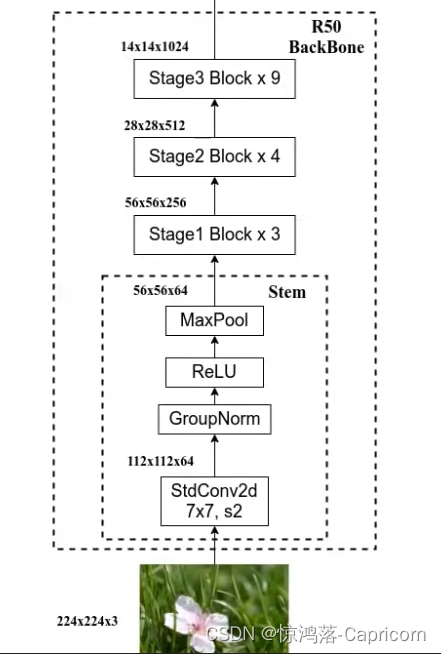
6.1 Hybird ViT
先用Resnet50特征提取,再用ViT进一步处理分类。

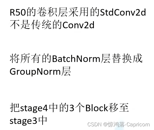
其中Resnet50部分做出了一些修改;
epoch较多时,混合模型模型反而效果不如纯正的ViT。

