小蓝xlanll

这个屌丝很懒，什么也没留下！

热门标签

七月论文审稿GPT第4版：通过paper-review数据集微调Mixtral-8x7b，对GPT4胜率超过80%

作者：小蓝xlanll | 2024-04-16 08:14:18

踩

前言

在此之前，我司论文审稿项目组已经通过我司处理的paper-review数据集，分别微调了RWKV、llama2、gpt3.5 16K、llama2 13b、Mistral 7b instruct、gemma 7b

七月论文审稿GPT第1版：通过3万多篇paper和10多万的review数据微调RWKV
七月论文审稿GPT第2版：用一万多条paper-review数据集微调LLaMA2 7B最终反超GPT4
七月论文审稿GPT第2.5和第3版：分别微调GPT3.5、Llama2 13B以扩大对GPT4的优势
七月论文审稿GPT第3.2版和第3.5版：通过paper-review数据集分别微调Mistral、gemma

虽然其中gemma 7b已经把对GPT4-1106的胜率达到了78%，但效果提升是永无止境的，故继续折腾，在本文要介绍的第4版我们则微调mixtral 8x7b(关于mixtral 87的介绍，详见此文：从Mistral 7B到MoE模型Mixtral 8x7B的全面解析：从原理分析到代码解读)，且首次把对GPT4-1106的胜率达到了80%

然虽然结果是令人振奋的，但过程却是充满曲折，我24年3.13拉的群：七月审稿GPT：微调Mixtral-8x7b，可直到4月2日，整个mixtral 8×7b的微调过程才基本完结，其中做了这么几件事

一方面，不染、吴同学、鸿飞等人一开始通过llama factory微调mixtral 8×7b
三方面，贾斯丁通过xtuner微调mixtral 8×7b
3.14，便把1.5K的数据跑通了(最早的1.5k数据，1张80g a100和a40都试过)，后面则继续用5K的数据、15K的数据分别微调mixtral 8×7b
三方面，三太子尝试通过Swift微调mixtral 8×7b
swift，跟xtuner(上海AI实验室推出)、llama-factory都差不多，都属于高度封装
且大部分教学都用的开源数据，然后定义了template，dataset，model
但这条路线暂时还没有走通，总的来说，swift目前用起来还不够顺手

第一部分通过llama factory微调mixtral 8x7b

1.1 模型训练：最终通过4张48G的A40跑15K数据

Mixtral-8x7b地址：魔搭社区

GitHub: hiyouga/LLaMA-Factory: Unify Efficient Fine-tuning of 100+ LLMs (github.com)

1.1.1 环境配置


git clone https://github.com/hiyouga/LLaMA-Factory.git
conda create -n llama_factory python=3.10
conda activate llama_factory
cd /root/path/LLaMA-Factory
pip install -r requirements.txt

有些得单独版本对齐，不染使用的是cuda11.8


pip install torch==2.1.2 torchvision==0.16.2 torchaudio==2.1.2 --index-url https://download.pytorch.org/whl/cu118
pip install bitsandbytes==0.41.3
# 下载对应版本 https://github.com/Dao-AILab/flash-attention/releases
pip install flash_attn-2.5.2+cu118torch2.1cxx11abiFALSE-cp310-cp310-linux_x86_64.whl

1.1.2 训练代码：分别基于1.5K、15K数据训练

一开始在1张80G的A800上训练，通过1.5K的少部分数据小试牛刀下，从而在终端执行代码：


python src/train_bash.py \
    --stage sft \
    --do_train True \
    --model_name_or_path /root/weights/Mixtral-8x7B-Instruct-v0.1 \
    --finetuning_type lora \
	--quantization_bit 4 \
    --template mistral \
    --flash_attn True \
    --dataset_dir data \
    --dataset paper_review_data \
    --cutoff_len 12288 \
    --learning_rate 5e-05 \
    --num_train_epochs 3.0 \
    --max_samples 1000000 \
    --per_device_train_batch_size 16 \
    --gradient_accumulation_steps 1 \
    --lr_scheduler_type cosine \
    --max_grad_norm 0.3 \
    --logging_steps 10 \
	--warmup_steps 0 \
	--lora_rank 128 \
    --save_steps 1000 \
    --lora_dropout 0.05 \
    --lora_target q_proj,o_proj,k_proj,v_proj,down_proj,gate_proj,up_proj \
    --output_dir saves/Mixtral-8x7B-Chat/lora/train_2024-03-23 \
    --fp16 True \
    --plot_loss True

之后，在4张48G的A40上跑全部的15K数据，从而在终端执行代码：


deepspeed --num_gpus 4 --master_port=9907 src/train_bash.py \
	--deepspeed ds_z3_config.json \
    --stage sft \
    --do_train True \
    --model_name_or_path /root/weights/Mixtral-8x7B-Instruct-v0.1 \
    --finetuning_type lora \
	--overwrite_cache \
    --template mistral \
    --flash_attn True \
    --dataset_dir data \
    --dataset paper_review_data_15565 \
    --learning_rate 5e-05 \
    --num_train_epochs 3.0 \
    --cutoff_len 32768 \
    --max_samples 1000000 \
    --per_device_train_batch_size 1 \
    --gradient_accumulation_steps 8 \
    --lr_scheduler_type cosine \
    --max_grad_norm 0.3 \
    --logging_steps 10 \
	--warmup_steps 0 \
	--lora_rank 32 \
    --save_steps 100 \
    --lora_dropout 0.05 \
    --lora_target q_proj,o_proj,k_proj,v_proj \
    --output_dir saves/Mixtral-8x7B-Chat/lora/train_2024-03-30 \
    --fp16 True \
    --plot_loss True

且设置ds_z3_config.json：


{
  "train_batch_size": "auto",
  "train_micro_batch_size_per_gpu": "auto",
  "gradient_accumulation_steps": "auto",
  "gradient_clipping": "auto",
  "zero_allow_untested_optimizer": true,
  "fp16": {
    "enabled": "auto",
    "loss_scale": 0,
    "loss_scale_window": 1000,
    "initial_scale_power": 16,
    "hysteresis": 2,
    "min_loss_scale": 1
  },
  "bf16": {
    "enabled": "auto"
  },
  "zero_optimization": {
    "stage": 3,
    "overlap_comm": true,
    "contiguous_gradients": true,
    "sub_group_size": 1e9,
    ..
    # 完整代码见七月官网的：大模型商用项目之审稿GPT微调实战
  }
}

1.2 模型推理

1.2.1 部署API接口

这里使用lora执行src/api_demo.py时会出现一个问题：

NotImplementedError: Cannot copy out of meta tensor; no data! · Issue #2940 · hiyouga/LLaMA-Factory (github.com)

解决方案：训练时使用了--quantization_bit 4 和 --flash_attn True，这里也要使用统一的才行。


CUDA_VISIBLE_DEVICES=0 API_PORT=8000 python src/api_demo.py \
    --model_name_or_path /root/weights/Mixtral-8x7B-Instruct-v0.1 \
    --adapter_name_or_path /root/path/saves/Mixtral-8x7B-Chat/lora/train_train_2024-03-23 \
    --template mistral \
    --finetuning_type lora \
    --quantization_bit 4 \
	--flash_attn True

推理所需显存为34318MiB

1.2.2 调用API接口

更多见七月的《大模型商用项目之审稿GPT微调实战》

第二部分通过xtuner微调mixtral 8x7b

如贾斯汀所说

v1代表5K数据 + qlora，用的 1张80G的A100
v2代表15K数据 + qlora，用的8张40G的A100
v3代表15K+全量微调+没开量化+纯bf16，用的8张40G的A100

2.1 微调之前的准备：Xtuner安装、数据格式修改、数据组织、config

2.1.1 框架Xtuner的安装

Xtuner安装地址：https://github.com/InternLM/xtuner/blob/main/README_zh-CN.md

快速安装步骤如下

推荐使用 conda 先构建一个 Python-3.10 的虚拟环境


conda create --name xtuner-env python=3.10 -y
conda activate xtuner-env

通过 pip 安装 XTuner：

pip install -U xtuner

亦可集成 DeepSpeed 安装：

pip install -U 'xtuner[deepspeed]'

当然，也可以从源码安装 XTuner：


git clone https://github.com/InternLM/xtuner.git
cd xtuner
pip install -e '.[all]'

需要额外安装flash attn


# Mixtral requires flash-attn
pip install flash-attn
# install the latest transformers
 
pip install -U transformers

2.1.2 数据格式修改

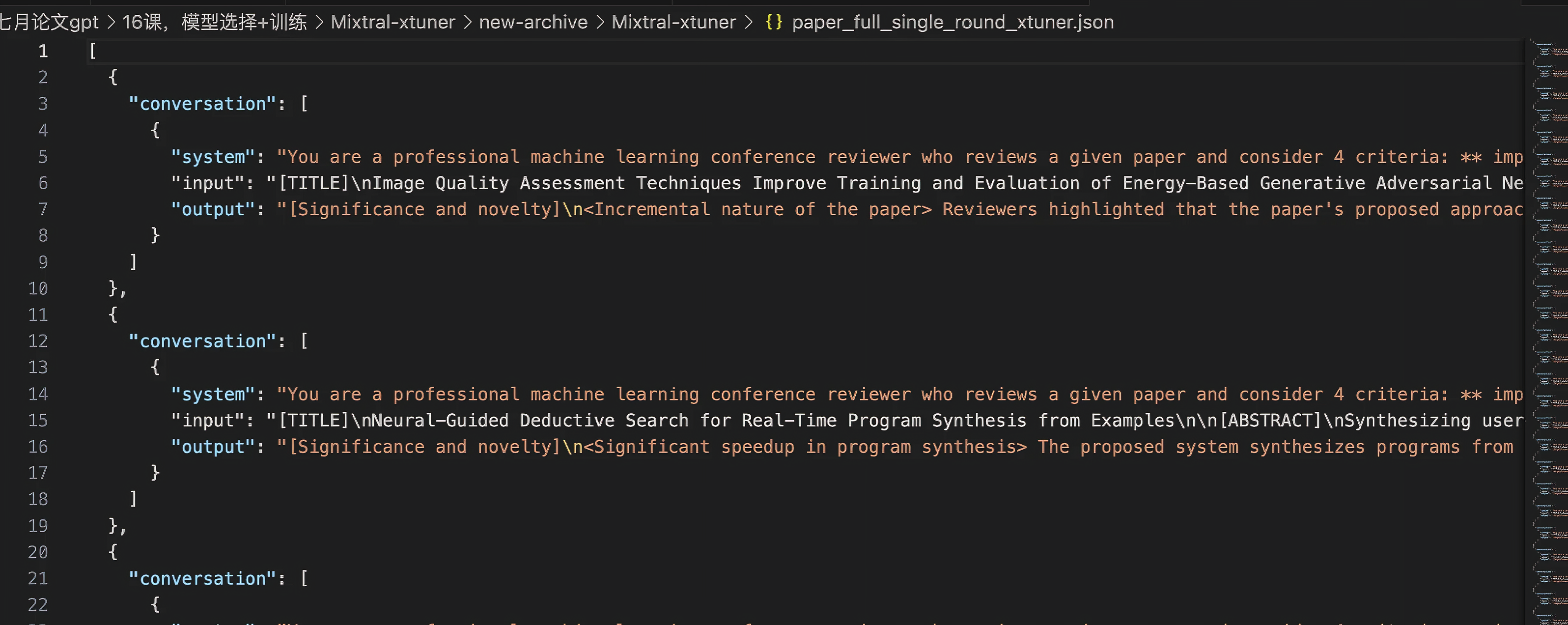
xtuner要求自定义数据集，我们的数据是input-output两个键，需要改成下面格式：


[{
    "conversation":[
        {
            "system": "xxx",
            "input": "xxx",
            "output": "xxx"
        }
    ]
},
{
    "conversation":[
        {
            "system": "xxx",
            "input": "xxx",
            "output": "xxx"
        }
    ]
}]

这是xtuner要求的自定义的单轮对话数据格式，我们也是单轮对话，也就是说每次的input-output前面都加上" you are a professional machine xxx......" 即可，比如

system_prompt = "You are a professional machine learning conference reviewer who reviews a given paper and considers 4 criteria: ** importance and novelty **, ** potential reasons for acceptance **, ** potential reasons for rejection **, and ** suggestions for improvement **. The given paper is as follows."
或
system_prompt = "You are a professional machine learning conference reviewer who reviews a given paper and considers 4 criteria: [Significance and novelty], [Potential reasons for acceptance], [Potential reasons for rejection], and [Suggestions for improvement]. For each criterion, provide random number of supporting points derived from the paper's content. And for each supporting point, use the format: '<title of supporting point>' followed by a detailed explanation. Your response should only include your reviews only, which means always start with [Significance and novelty], dont' repeat the given paper and output things other than your reviews in required format. The paper is given as follows:"

具体实现时，可以通过写一个convert_jsonl_to_xtuner_format的函数(代码见七月大模型商用项目之审稿GPT微调实战)，然后做到如下效果

2.1.3 修改数据组织格式

在xtuner/xtuner/dataset/utils.py 中，修改这个encode_fn，实现截断操作(使用which xtuner，一路找到sitepackages中这个文件)：

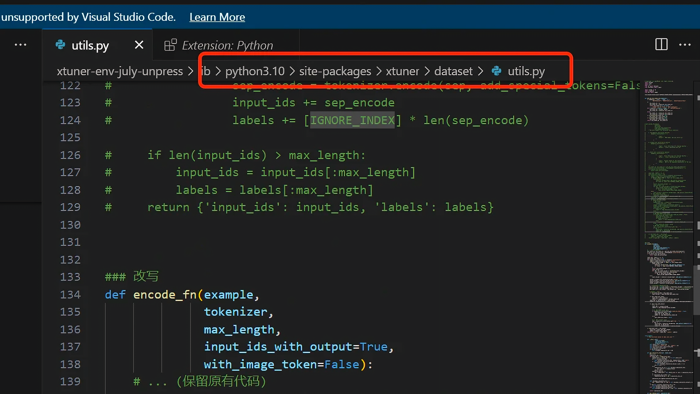
直接把原先的comment掉，替换成下面的代码(encode_fn代码见七月大模型商用项目之审稿GPT微调实战)

2.1.4 config

xtuner的config都是用py文件的，我们要选择适合我们特定模型的config模板，并且因为自定义了数据集，也要对config进行修改(参考：xtuner/docs/zh_cn/user_guides/single_turn_conversation.md at 59834032c82d39994c13252aea9b00011d1b2457 · InternLM/xtuner · GitHub)

找到模板
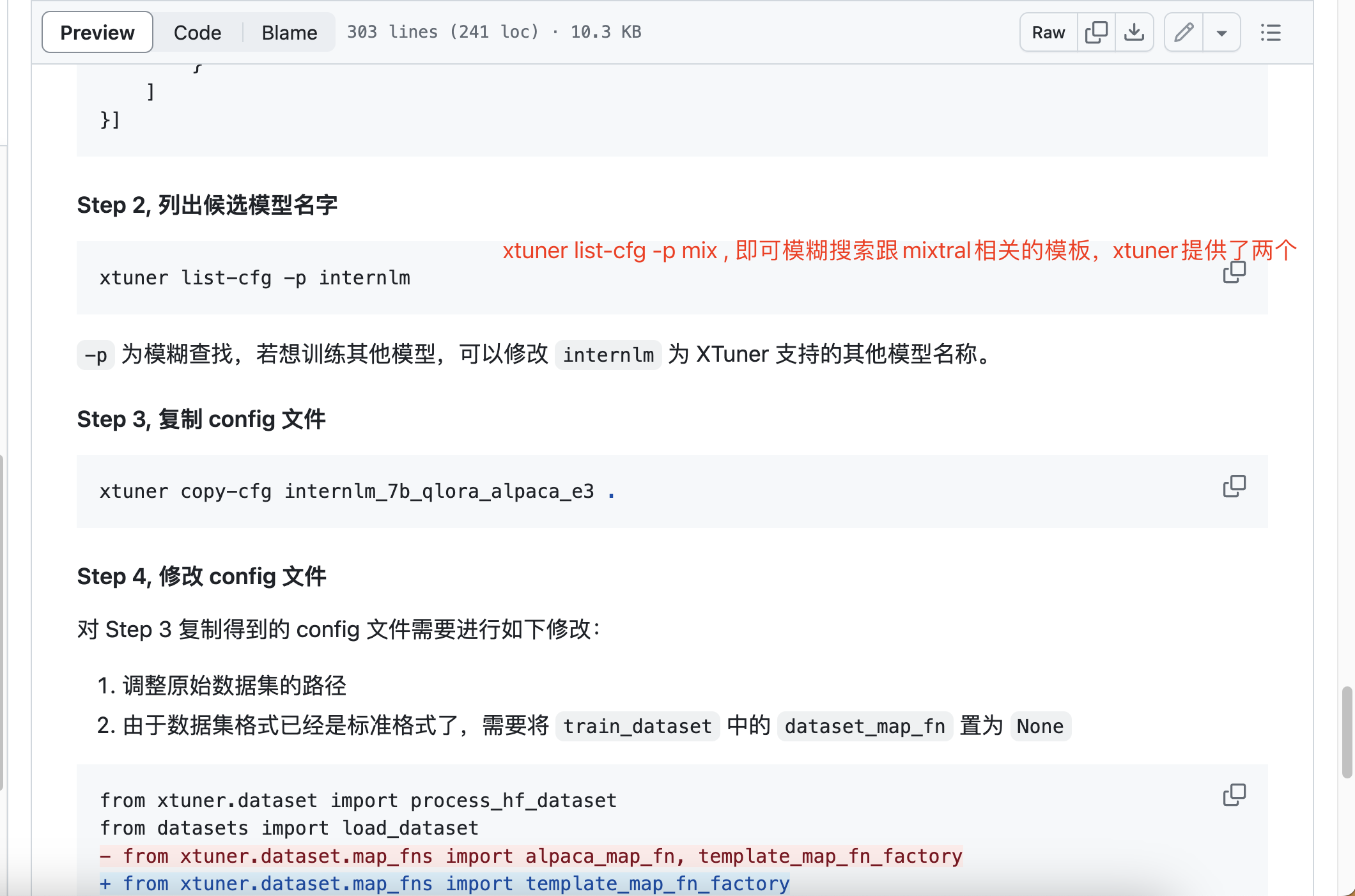
使用下面命令，会复制一份mixtral_8x7b_instruct_qlora_oasst1_e3.py这个config，然后我们基于这个模板去修改参数(下面这个代码会把xtuner提供的mixtral_8x7b_instruct_qlora_oasst1_e3.py 复制一份到你当前目录下)：
```
xtuner copy-cfg mixtral_8x7b_instruct_qlora_oasst1_e3 .
```
由于自定义数据集，config中几个关键点按照xtuner所提示的进行修改，减号代表删除这一行，加号代表增加这一行：

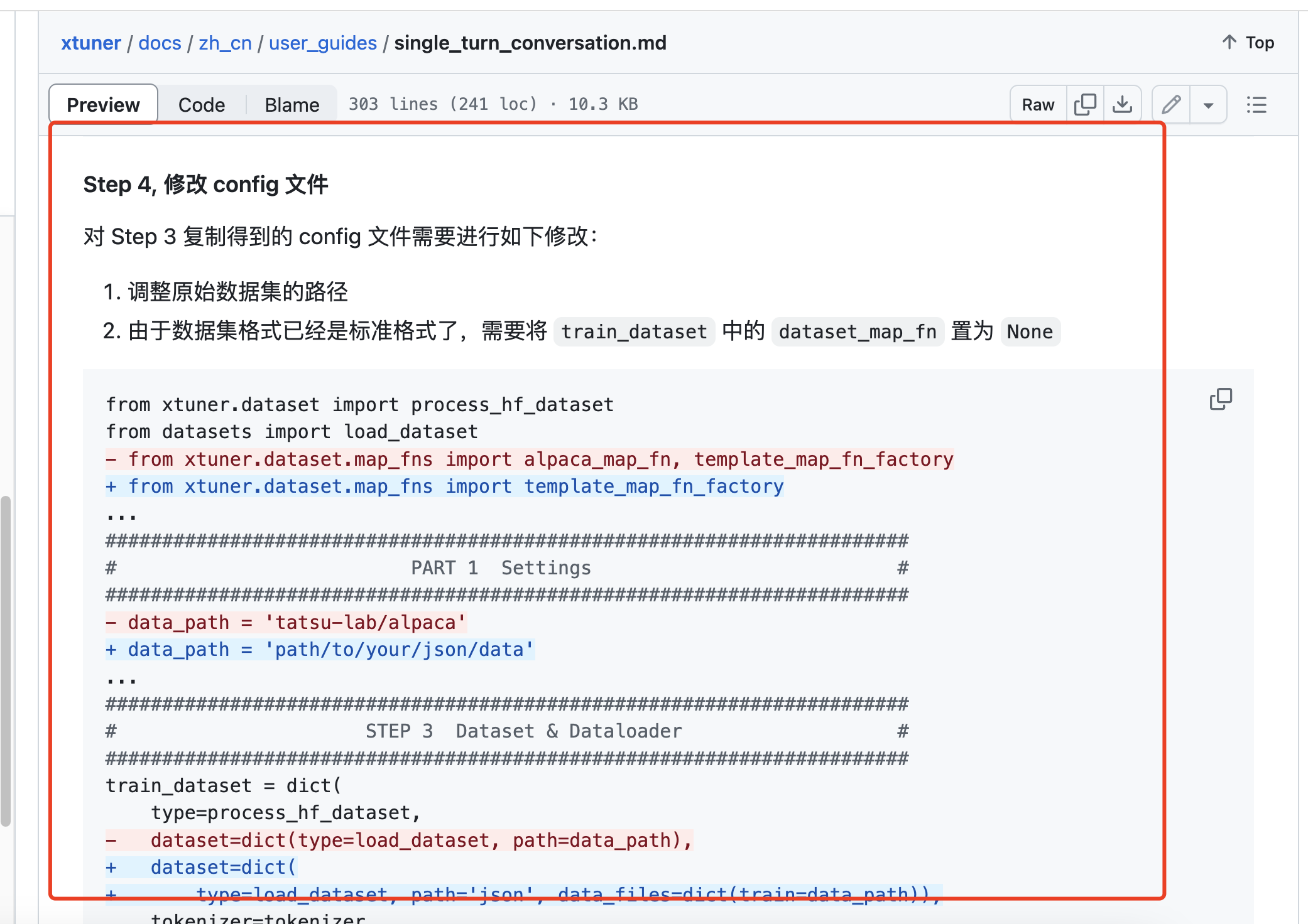
另外，模型需要自行下载，贾斯汀是租的国外gpu，因此直接从huggingface 去git clone的，一小时下完，然而mixtral 8x7b 除了safetensor还有pt文件，直接gitclone 会下载两份很大，建议大家想办法只下载safetenor和其他config即可

2.1.5 最终config.py展示

具体模板的各个参数是什么，请参考：xtuner/docs/zh_cn/user_guides/config.md at 59834032c82d39994c13252aea9b00011d1b2457 · InternLM/xtuner · GitHub (当然他这个解释的也不太细，尽量去issue或这个github库中搜索相关定义和关键字)

在v1中，使用5000条数据进行微调，最终贾斯汀用到的mixtral_8x7b_instruct_qlora_oasst1_e3_2.py 模板见七月大模型商用项目之审稿GPT微调实战
模板中的evaluation_inputs如下所示，其代表训练中间去evaluate的时候的输入，贾斯汀这边直接复制了几个论文的string，也可以不加


evaluation_inputs = [ 
                     
                     """
                     [TITLE]\nYaRN: Efficient Context Window Extension of Large Language Models\n\n[ABSTRACT]\nRotary Position Embeddings (RoPE) have been shown to effectively encode posi- tional information in transformer-based language models. However, these models fail to generalize past the sequence length they were trained on. We present YaRN (Yet another RoPE extensioN method), a compute-efficient method to extend the context window of such models, requiring 10x less tokens and 2.5x less training steps than previous methods. Using YaRN, we show that LLaMA models can effectively utilize and extrapolate to context lengths much longer than their original pre-training would allow, while also surpassing previous the state-of-the-art at context window extension. In addition, we demonstrate that YaRN exhibits the capability to extrapolate beyond the limited context of a fine-tuning dataset. The models fine-tuned using YaRN has been made available and reproduced online up to 128k context length at https://github.com/jquesnelle/yarn.\n\n[CAPTIONS]\nFigure 1: Sliding window perplexity (S = 256) of ten 128k Proof-pile documents truncated to evaluation context window size\nTable 1: Sliding window perplexity (S = 256) of ten 128k Proof-pile documents over Llama-2 extended via PI, NTK and YaRN\nTable 2: Sliding window perplexity (S = 256) of ten 128k Proof-pile documents truncated to evaluation context window size\nTable 3: Performance of context window extensions methods on the Hugging Face Open LLM benchmark suite compared with original Llama 2 baselines\n\n[CONTENT]\nSection Title: Introduction\n  Introduction Transformer-based Large Language Models[40] (LLMs) have become the near-ubiquitous choice for many natural language processing (NLP) tasks where long-range abilities such as in-context learning (ICL) has been crucial. In performing the NLP tasks, the maximal length of the sequences (the context window) determined by its training processes has been one of the major limits of a pretrained LLM. Being able to dynamically extend the context window via a small amount of fine-tuning (or without fine-tuning) has become more and more desirable. To this end, the position encodings of transformers are the center of the discussions. The original Transformer architecture used an absolute sinusoidal position encoding, which was later improved to a learnable absolute position encoding [15]. Since then, relative positional encoding schemes [32] have further increased the performance of Transformers. Currently, the most popular relative positional encodings are T5 Relative Bias [30], RoPE [34], XPos [35], and ALiBi [27]. One reoccurring limitation with positional encodings is the inability to generalize past the context window seen during training. While some methods such as ALiBi are able to do limited generalization, none are able to generalize to sequences significantly longer than their pre-trained length [22]. Some works have been done to overcome such limitation. [9] and concurrently [21] proposed to extend the context length by slightly modifying RoPE via Position Interpolation (PI) and fine-tuning on a small amount of data. As an alternative, [6] proposed the \"NTK-aware\" interpolation by taking the loss of high frequency into account. Since then, two improvements of the \"NTK-aware\" interpolation have been proposed, with different emphasis: • the \"Dynamic NTK\" interpolation method [14] for pre-trained models without fine-tuning. • the \"NTK-by-parts\" interpolation method [7] which performs the best when fine-tuned on a small amount of longer-context data. The \"NTK-aware\" interpolation and the \"Dynamic NTK\" interpolation have already seen their presence in the open-source models such as Code Llama [31] (using \"NTK-aware\" interpolation) and Qwen 7B [2] (using \"Dynamic NTK\"). In this paper, in addition to making a complete account of the previous unpublished works on the \"NTK-aware\", the \"Dynamic NTK\" and the \"NTK-by-part\" interpolations, we present YaRN (Yet another RoPE extensioN method), an improved method to efficiently extend the context window of models trained with Rotary Position Embeddings (RoPE) including the LLaMA [38], the GPT- NeoX [5], and the PaLM [10] families of models. YaRN reaches state-of-the-art performances in context window extensions after fine-tuning on less than ∼0.1% of the original pre-training data. In the meantime, by combining with the inference-time technique called Dynamic Scaling, the Dynamic-YaRN allows for more than 2x context window extension without any fine-tuning.\n\nSection Title: Background and Related Work\n  Background and Related Work\n\nSection Title: Rotary Position Embeddings\n  Rotary Position Embeddings The basis of our work is the Rotary Position Embedding (RoPE) introduced in [34]. We work on a hidden layer where the set of hidden neurons are denoted by D. Given a sequence of vectors x 1 , · · · , x L ∈ R |D| , following the notation of [34], the attention layer first converts the vectors into the query vectors and the key vectors: Next, the attention weights are calculated as softmax( q T m k n |D| ), (2) where q m , k n are considered as column vectors so that q T m k n is simply the Euclidean inner product. In RoPE, we first assume that |D| is even and identify the embedding space and the hidden states as complex vector spaces: R |D| ∼ = C |D|/2 where the inner product q T k becomes the real part of the standard Hermitian inner product Re(q * k). More specifically, the isomorphisms interleave the real part and the complex part To convert embeddings x m , x n into query and key vectors, we are first given R-linear operators In complex coordinates, the functions f q , f k are given by where θ = diag(θ 1 , · · · , θ |D|/2 ) is the diagonal matrix with θ d = b −2d/|D| and b = 10000. This way, RoPE associates each (complex-valued) hidden neuron with a separate frequency θ d . The benefit of doing so is that the dot product between the query vector and the key vector only depends on the relative distance m − n as follows In real coordinates, the RoPE can be written using the following function\n\nSection Title: Position Interpolation\n  Position Interpolation As language models are usually pre-trained with a fixed context length, it is natural to ask how to extend the context length by fine-tuning on relatively less amount of data. For language models using RoPE as the position embedding, Chen et al. [9], and concurrently kaiokendev [21] proposed the Position Interpolation (PI) to extend the context length beyond the pre-trained limit. While a direct extrapolation does not perform well on sequences w 1 , · · · , w L with L larger than the pre-trained limit, they discovered that interpolating the position indicies within the pre-trained limit works well with the help of a small amount of fine-tuning. Specifically, given a pre-trained language model with RoPE, they modify the RoPE by f ′ W (x m , m, θ d ) = f W x m , mL L ′ , θ d , (10) where L ′ > L is a new context window beyond the pre-trained limit. With the original pre-trained model plus the modified RoPE formula, they fine-tuned the language model further on several orders of magnitude fewer tokens (a few billion in Chen et al. [9]) and successfully acheived context window extension.\n\nSection Title: Additional Notation\n  Additional Notation The ratio between the extended context length and the original context length has been of special importance, and we introduce the notation s defined by s = L ′ L , (11) and we call s the scale factor. We also rewrite and simplify Eq. 10 into the following general form: where g(m), h(θ d ) are method-dependent functions. For PI, we have g(m) = m/s, h(θ d ) = θ d . In the subsequent sections, when we introduce a new interpolation method, we sometimes only specify the functions g(m) and h(θ d ). Additionally, we define λ d as the wavelength of the RoPE embedding at d-th hidden dimension: The wavelength describes the length of tokens needed in order for the RoPE embedding at dimension d to perform a full rotation (2π). Given that some interpolation methods (eg. PI) do not care about the wavelength of the dimensions, we will refer to those methods as \"blind\" interpolation methods, while others do (eg. YaRN), which we will classify as \"targeted\" interpolation methods.\n\nSection Title: Related work\n  Related work ReRoPE [33] also aims to extend the context size of existing models pre-trained with RoPE, and claims \"infinite\" context length without needing any fine-tuning. This claim is backed by a monotonically decreasing loss with increasing context length up to 16k on the Llama 2 13B model. It achieves context extension by modifying the attention mechanism and thus is not purely an embedding interpolation method. Since it is currently not compatible with Flash Attention 2 [13] and requires two attention passes during inference, we do not consider it for comparison. Concurrently with our work, LM-Infinite [16] proposes similar ideas to YaRN, but focuses on \"on-the- fly\" length generalization for non-fine-tuned models. Since they also modify the attention mechanism of the models, it is not an embedding interpolation method and is not immediately compatible with Flash Attention 2.\n\nSection Title: Methodology\n  Methodology Whereas PI stretches all RoPE dimensions equally, we find that the theoretical interpolation bound described by PI [9] is insufficient at predicting the complex dynamics between RoPE and the LLM's internal embeddings. In the following subsections, we describe the main issues with PI we have individually identified and solved, so as to give the readers the context, origin and justifications of each method which we use in concert to obtain the full YaRN method.\n\nSection Title: Loss of High Frequency information - \"NTK-aware\" interpolation\n  Loss of High Frequency information - \"NTK-aware\" interpolation If we look at RoPE only from an information encoding perspective, it was shown in [36], using Neural Tangent Kernel (NTK) theory, that deep neural networks have trouble learning high frequency information if the input dimension is low and the corresponding embeddings lack high frequency components. Here we can see the similarities: a token's positional information is one-dimensional, and RoPE expands it to an n-dimensional complex vector embedding. RoPE closely resembles Fourier Features [36] in many aspects, as it is possible to define RoPE as a special 1D case of a Fourier Feature. Stretching the RoPE embeddings indiscriminately results in the loss of important high frequency details which the network needs in order to resolve tokens that are both very similar and very close together (the rotation describing the smallest distance needs to not be too small for the network to be able to detect it). We hypothesise that the slight increase of perplexity for short context sizes after fine-tuning on larger context sizes seen in PI [9] might be related to this problem. Under ideal circumstances, there is no reason that fine-tuning on larger context sizes should degrade the performance of smaller context sizes. In order to resolve the problem of losing high frequency information when interpolating the RoPE embeddings, the \"NTK-aware\" interpolation was developed in [6]. Instead of scaling every dimension of RoPE equally by a factor s, we spread out the interpolation pressure across multiple dimensions by scaling high frequencies less and low frequencies more. One can obtain such a transformation in many ways, but the simplest would be to perform a base change on the value of θ. More precisely, following the notations set out in Section 2.3, we define the \"NTK-aware\" interpola- tion scheme as follows (see the Appendix A.1 for the details of the deduction).\n\nSection Title: Definition 1\n  Definition 1 The \"NTK-aware\" interpolation is a modification of RoPE by using Eq. 12 with the following functions. Given the results from [6], this method performs much better at extending the context size of non-fine- tuned models compared to PI [9]. However, one major disadvantage of this method is that given it is not just an interpolation scheme, some dimensions are slightly extrapolated to \"out-of-bound\" values, thus fine-tuning with \"NTK-aware\" interpolation [6] yields inferior results to PI [9]. Furthermore, due to the \"out-of-bound\" values, the theoretical scale factor s does not accurately describe the true context extension scale. In practice, the scale value s has to be set higher than the expected scale for a given context length extension. We note that shortly before the release of this article, Code Llama [31] was released and uses \"NTK-aware\" scaling by manually scaling the base b to 1M.\n\nSection Title: Loss of Relative Local Distances - \"NTK-by-parts\" interpolation\n  Loss of Relative Local Distances - \"NTK-by-parts\" interpolation In the case of blind interpolation methods like PI and \"NTK-aware\" interpolation, we treat all the RoPE hidden dimensions equally (as in they have the same effect on the network). However, there are strong clues that point us towards the need for targeted interpolation methods. In this section, we think heavily in terms of the wavelengths λ d defined in Eq. 13 in the formula of RoPE. For simplicity, we omit the subscript d in λ d and the reader is encouraged to think about λ as the wavelength of an arbitrary periodic function. One interesting observation of RoPE embeddings is that given a context size L, there are some dimensions d where the wavelength is longer than the maximum context length seen during pretraining (λ > L), this suggests that some dimensions' embeddings might not be distributed evenly in the rotational domain. In such cases, we presume having all unique position pairs implies that the absolute positional information remains intact. On the contrary, when the wavelength is short, only relative positional information is accessible to the network. Moreover, when we stretch all the RoPE dimensions either by a scale s or using a base change b ′ , all tokens become closer to each other, as the dot product of two vectors rotated by a lesser amount is bigger. This scaling severely impairs a LLM's ability to understand small and local relationships between its internal embeddings. We hypothesize that such compression leads to the model being confused on the positional order of close-by tokens, and consequently harming the model's abilities. In order to remedy this issue, given the two previous observations that we have found, we choose not to interpolate the higher frequency dimensions at all while always interpolating the lower frequency dimensions. In particular, • if the wavelength λ is much smaller than the context size L, we do not interpolate; • if the wavelength λ is equal to or bigger than the context size L, we want to only interpolate and avoid any extrapolation (unlike the previous \"NTK-aware\" method); • dimensions in-between can have a bit of both, similar to the \"NTK-aware\" interpolation. As a result, it is more convenient to introduce the ratio r = L λ between the original context size L and the wavelength λ. In the d-th hidden state, the ratio r depends on d in the following way: In order to define the boundary of the different interpolation strategies as above, we introduce two extra parameters α, β. All hidden dimensions d where r(d) < α are those where we linearly interpolate by a scale s (exactly like PI, avoiding any extrapolation), and the d where r(d) > β are those where we do not interpolate at all. Define the ramp function γ to be With the help of the ramp function, the \"NTK-by-parts\" method can be described as follows.\n\nSection Title: Definition 2\n  Definition 2 The \"NTK-by-parts\" interpolation is a modification of RoPE by using Eq. 12 with the following functions 4 . The values of α and β should be tuned on a case-by-case basis. For example, we have found experimentally that for the Llama family of models, good values for α and β are α = 1 and β = 32. Using the techniques described in this section, a variant of the resulting method was released under the name \"NTK-by-parts\" interpolation [7]. This improved method performs better than the previous PI [9] and \"NTK-aware\" 3.1 interpolation methods, both with non-fine-tuned models and with fine-tuned models, as shown in [7].\n\nSection Title: Dynamic Scaling - \"Dynamic NTK\" interpolation\n  Dynamic Scaling - \"Dynamic NTK\" interpolation In a lot of use cases, multiple forward-passes are performed with varying sequence lengths from 1 to the maximal context size. A typical example is the autoregressive generation where the sequence lengths increment by 1 after each step. There are two ways of applying an interpolation method that uses a scale factor s (including PI, \"NTK-aware\" and \"NTK-by-parts\"): 1. Throughout the whole inference cycle, the embedding layer is fixed including the scale factor s = L ′ /L where L ′ is the fixed number of extended context size. 2. In each forward-pass, the position embedding updates the scale factor s = max(1, l ′ /L) where l ′ is the sequence length of the current sequence. The problem of (1) is that the model may experience a performance discount at a length less than L and an abrupt degradation when the sequence length is longer than L ′ . But by doing Dynamic Scaling as (2), it allows the model to gracefully degrade instead of immediately breaking when hitting the trained context limit L ′ . We call this inference-time method the Dynamic Scaling method. When it is combined with \"NTK-awared\" interpolation, we call it \"Dynamic NTK\" interpolation. It first appeared in public as a reddit post in [14]. One notable fact is that the \"Dynamic NTK\" interpolation works exceptionally well on models pre- trained on L without any finetuning (L ′ = L). This is supported by the experiment in Appendix B.3. Often in the repeated forward-passes, the kv-caching [8] is applied so that we can reuse the previous key-value vectors and improve the overall efficiency. We point out that in some implementations when the RoPE embeddings are cached, some care has to be taken in order to modify it for Dynamic Scaling with kv-caching. The correct implementation should cache the kv-embeddings before applying RoPE, as the RoPE embedding of every token changes when s changes.\n\nSection Title: YaRN\n  YaRN In addition to the previous interpolation techniques, we also observe that introducing a temperature t on the logits before the attention softmax has a uniform impact on perplexity regardless of the data sample and the token position over the extended context window (See Appendix A.2). More precisely, instead of Eq. 2, we modify the computation of attention weights into The reparametrization of RoPE as a set of 2D matrices has a clear benefit on the implementation of this attention scaling: we can instead use a \"length scaling\" trick which scales both q m and k n by a constant factor 1/t by simply scaling the complex RoPE embeddings by the same amount. With this, YaRN can effectively alter the attention mechanism without modifying its code. Furthermore, it has zero overhead during both inference and training, as RoPE embeddings are generated in advance and are reused for all forward passes. Combining it with the \"NTK-by-parts\" interpolation, we have the YaRN method.\n\nSection Title: Definition 3\n  Definition 3 By the \"YaRN method\", we refer to a combination of the attention scaling in Eq. 21 and the \"NTK-by-parts\" interpolation introduced in Section 3.2. For LLaMA and Llama 2 models, we recommend the following values: The equation above is found by fitting 1/t at the lowest perplexity against the scale extension by various factors s using the \"NTK-by-parts\" method (Section 3.2) on LLaMA 7b, 13b, 33b and 65b models without fine-tuning. We note that the same values of t also apply fairly well to Llama 2 models (7b, 13b and 70b). It suggests that the property of increased entropy and the temperature constant t may have certain degree of \"universality\" and may be generalizable across some models and training data. The YaRN method combines all our findings and surpasses all previous methods in both fine-tuned and non-fine-tuned scenarios. Thanks to its low footprint, YaRN allows for direct compatibility with libraries that modify the attention mechanism such as Flash Attention 2 [13].\n\nSection Title: Experiments\n  Experiments We show that YaRN successfully achieves context window extension of language models using RoPE as its position embedding. Moreover, this result is achieved with only 400 training steps, representing approximately 0.1% of the model's original pre-training corpus, a 10x reduction from Rozière et al. [31] and 2.5x reduction in training steps from Chen et al. [9], making it highly compute-efficient for training with no additional inference costs. We calculate the perplexity of long documents and score on established benchmarks to evaluate the resulting models, finding that they surpass all other context window extension methods. We broadly followed the training and evaluation procedures as outlined in [9].\n\nSection Title: Training\n  Training For training, we extended the Llama 2 [39] 7B and 13B parameter models. No changes were made to the LLaMA model architecture other than the calculation of the embedding frequencies as described in 3.4 with s = 16 and s = 32. We used a learning rate of 2 × 10 −5 with no weight decay and a linear warmup of 20 steps along with AdamW [24] β 1 = 0.9 and β 2 = 0.95. For s = 16 we fine-tuned for 400 steps with global batch size 64 using PyTorch [26] Fully Sharded Data Parallelism [42] and Flash Attention 2 [13] on the PG19 dataset [29] chunked into 64k segments bookended with the BOS and EOS token. For s = 32 we followed the same procedure, but started from the finished s = 16 checkpoint and trained for an additional 200 steps.\n\nSection Title: Extrapolation and Transfer Learning\n  Extrapolation and Transfer Learning In Code Llama [31], a dataset with 16k context was used with a scale factor set to s ≈ 88.6, which corresponds to a context size of 355k. They show that the network extrapolates up to 100k context without ever seeing those context sizes during training. Similar to 3.1 and Rozière et al. [31], YaRN also supports training with a higher scale factor s than the length of the dataset. Due to compute constraints, we test only s = 32 by further fine-tuning the s = 16 model for 200 steps using the same dataset with 64k context. We show in 4.3.1 that the s = 32 model successfully extrapolates up to 128k context using only 64k context during training. Unlike previous \"blind\" interpolation methods, YaRN is much more efficient at transfer learning when increasing the scale s. This demonstrates successful transfer learning from s = 16 to s = 32 without the network needing to relearn the interpolated embeddings, as the s = 32 model is equivalent to the s = 16 model across the entire context size, despite only being trained on s = 32 for 200 steps.\n\nSection Title: Evaluation\n  Evaluation The evaluations focus on three aspects: 1. the perplexity scores of fine-tuned models with extended context window, 2. the passkey retrieval task on fine-tuned models, 3. the common LLM benchmark results of fine-tuned models,\n\nSection Title: Long Sequence Language Modeling\n  Long Sequence Language Modeling To evaluate the long sequence language modeling performances, we use the GovReport [18] and Proof-pile [4] datasets both of which contain many long sequence samples. For all evaluations, the test splits of both datasets were used exclusively. All perplexity evaluations were calculated using the sliding window method from Press et al. [27] with S = 256. Firstly, we evaluated how the model performed as the context window increased. We selected 10 random samples from Proof-pile with at least 128k tokens each and evaluated the perplexity of each of these samples when truncated at 2k steps from a sequence length of 2k tokens through 128k tokens.  Table 1  shows a side-by-side comparison of Llama-2 model extended from 4096 to 8192 context length via PI (LLongMA-2 7b 5 ), \"NTK-aware\" and YaRN. Note that PI and \"NTK-aware\" models were trained using the methodology in Chen et al. [9], while YaRN used the same methodology but 2.5x less training steps and data, as described in 4. 5 LLongMA-2 7b [28] is fine-tuned from Llama-2 7b, trained at 8k context length with PI using the RedPajama dataset [12]. We further evaluated YaRN at the scale factor s = 16, 32 and compared them against a few open- source models fine-tuned from Llama-2 and extended to more than 32k context window such as Together.ai [37] and \"NTK-aware\" Code Llama [31]. The results are summarized in  Table 2  (with a more detailed plot in  Figure 1 ). We observe that the model exhibits strong performance across the entire targeted context size, with YaRN interpolation being the first method to successfully extend the effective context size of Llama 2 to 128k. Of particular note are the YaRN (s = 32) models, which show continued declining perplexity through 128k, despite the fine-tuning data being limited to 64k tokens in length, demonstrating that the model is able to generalize to unseen context lengths. Furthermore, in Appendix B.1, we show the results of the average perplexity on 50 untruncated GovReport documents with at least 16k tokens per sample evaluated on the setting of 32k maximal context window without Dynamic Scaling in Table 4. Similar to the Proof-pile results, the GovReport results show that fine-tuning with YaRN achieves good performance on long sequences.\n\nSection Title: Passkey Retrieval\n  Passkey Retrieval The passkey retrieval task as defined in [25] measures a model's ability to retrieve a simple passkey (i.e., a five-digit number) from amongst a large amount of otherwise meaningless text. For our evaluation of the models, we performed 10 iterations of the passkey retrieval task with the passkey placed at a random location uniformly distributed across the evaluation context window on different context window sizes ranging from 8k to 128k. Both 7b and 13b models fine-tuned using YaRN at 128k context size passes the passkey retrieval task with very high accuracy (> 99%) within the entire context window size. We show detailed results in Appendix B.2.\n\nSection Title: Standardized Benchmarks\n  Standardized Benchmarks The Hugging Face Open LLM Leaderboard [19] compares a multitude of LLMs across a standard- ized set of four public benchmarks. Specifically, we use 25-shot ARC-Challenge [11], 10-shot HellaSwag [41], 5-shot MMLU [17], and 0-shot TruthfulQA [23]. To test the degradation of model performance under context extension, we evaluated our models using this suite and compared it to established scores for the Llama 2 baselines as well as publicly available PI and \"NTK-aware\" models. The results are summarized in  Table 3 . We observe that there is minimal performance degradation between the YaRN models and their respective Llama 2 baselines. We also observe that there was on average a 0.49% drop in scores between the YaRN s = 16 and s = 32 models. From this we conclude that the the iterative extension from 64k to 128k results in negligible performance loss.\n\nSection Title: Conclusion\n  Conclusion In conclusion, we have shown that YaRN improves upon all existing RoPE interpolation methods and can act as a drop-in replacement to PI, with no downsides and minimal implementation effort. The fine-tuned models preserve their original abilities on multiple benchmarks while being able to attend to a very large context size. Furthermore, YaRN allows efficient extrapolation with fine- tuning on shorter datasets and can take advantage of transfer learning for faster convergence, both of which are crucial under compute-constrained scenarios. Finally, we have shown the effectiveness of extrapolation with YaRN where it is able to \"train short, and test long\".\n  The interpolation by linear ramp on h may have alternatives, such as a harmonic mean over θ d /s and θ d converted from a linear interpolation on wavelengths. The choice of h here was for the simplicity of implementation, but both would work. 
                     """]

在v2中使用的： mixtral_config_r64_w3_lr_alpha_system.py (代码见七月大模型商用项目之审稿GPT微调实战)
v3, 全量微调，精度也是默认的，应该是bf16 (代码见七月大模型商用项目之审稿GPT微调实战)

2.2 训练细节：从5K数据微调到15K数据+qlora微调、15K数据+全量微调

cd 到mixtral_8x7b_instruct_qlora_oasst1_e3_2.py 路径下，下面代码开启训练(5K数据时用的单卡A100 80g, 中间没有爆显存，维持在76G 左右)：


#v1
xtuner train mixtral_8x7b_instruct_qlora_oasst1_e3_2 --deepspeed deepspeed_zero2
 
# 可以自定义输出log到某个txt，也可以nohup， 看个人，
 
#v2 v3中用了8个40G的A100，命令小改
PROC_PER_NODE=8 xtuner train /mnt/llm_folder/July-Mixtral-files/mixtral_config_r64_w3_lr_alpha_system_full.py --deepspeed deepspeed_zero3_offload > output_lora_r64_w3_lr_alpha_system_full.txt 2>&1

2.2.1 v1：5K数据 + qlora

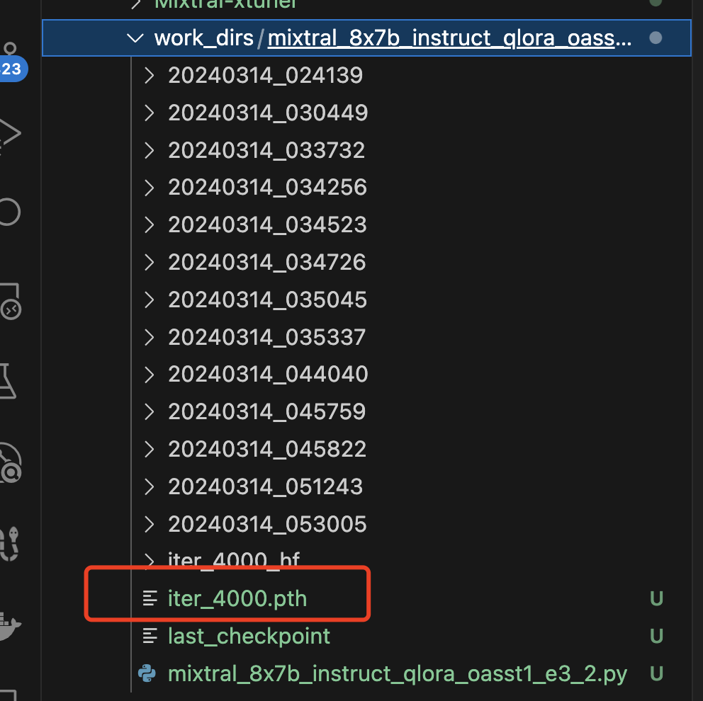
v1 中：2个epoch对应5190个steps，后来发现loss开始震荡，最终在4000个step的时候停止了

保存的adapter是：

2.2.2 v2：15K数据 + qlora

v2中保存逻辑类似

同样的，loss下降到1就不动了，咬咬牙3个epoch最终loss 到0.7：

2.2.3 v3：15K + 全量微调 + 没开量化 + 纯bf16

v3也是，几百个step就下降到1 了：

2.3 adapter的保存/合并

2.3.1 转化保存后的adapter

首先，需要把adapter从pth格式转化成bin格式，具体参考xtuner/README_zh-CN.md at 59834032c82d39994c13252aea9b00011d1b2457 · InternLM/xtuner · GitHub

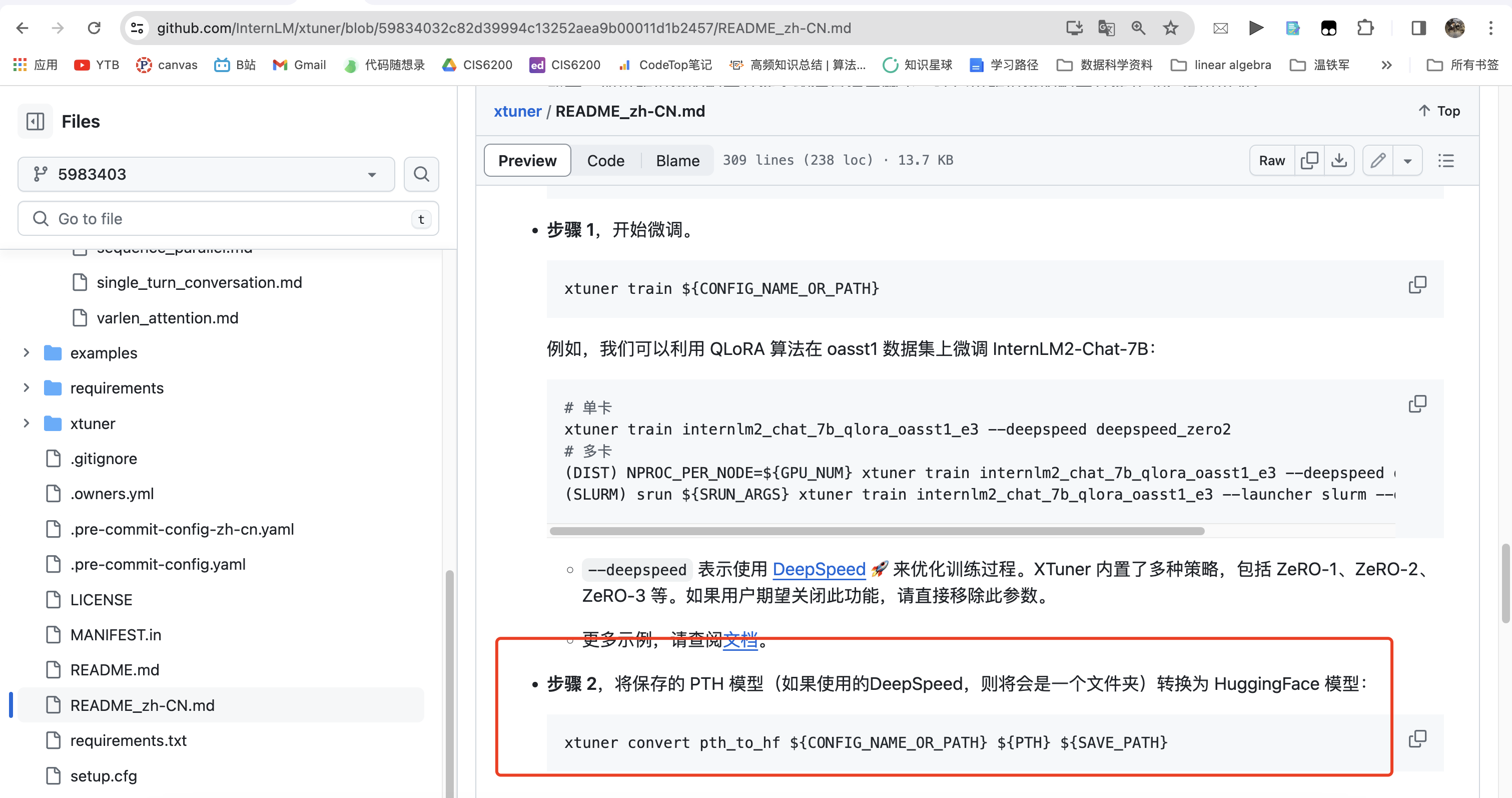
使用：

xtuner convert pth_to_hf ${CONFIG_NAME_OR_PATH} ${PTH} ${SAVE_PATH} --fp32

${CONFIG_NAME_OR_PATH} 就是你的mixtral_8x7b_instruct_qlora_oasst1_e3_2.py
${PTH} 和 ${SAVE_PATH} 就是你保存的iter_4000.pth和想要输出的路径
注意如果想要fp32精度，需要加上 --fp32, 默认是fp16. 建议添加，只是adapter大小会变成2倍

最终, v1/v2变成了bin文件(只有一个adapter)

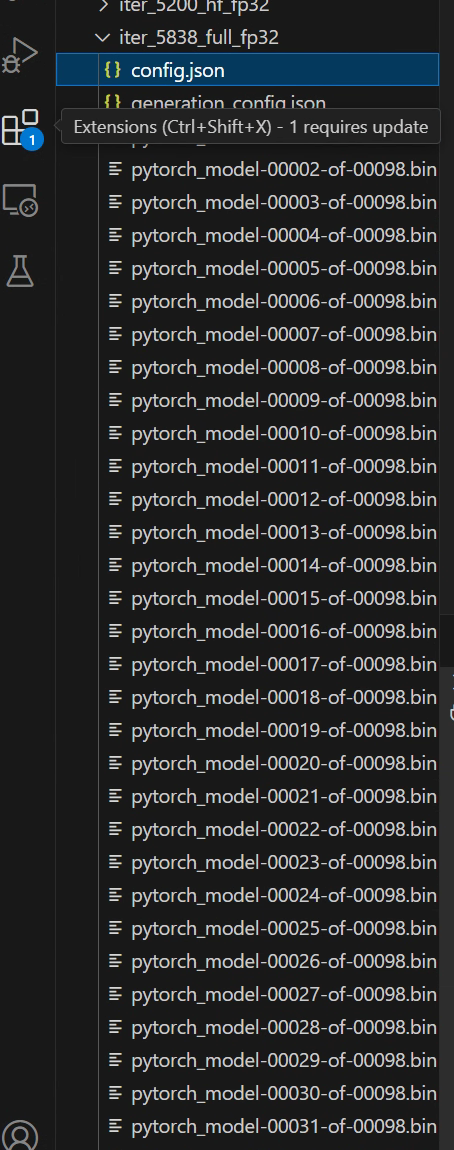
v3由于全量微调，不是adatper，直接是一个pth

因此只是把pth分成bin文件，转换为如下

2.3.2 合并模型和adapter(仅针对v1、v2)

参考：xtuner/README_zh-CN.md at 59834032c82d39994c13252aea9b00011d1b2457 · InternLM/xtuner · GitHub

注意，还要额外加 --device cpu，不然会OOM，因为训练时是用的 qlora ，所以显存够用

但 merge 时默认是在 gpu 上进行，此时加载的是模型全量参数，所以导致显存 OOM

因此使用下面的代码：


xtuner convert merge \
    ${NAME_OR_PATH_TO_LLM} \
    ${NAME_OR_PATH_TO_ADAPTER} \
    ${SAVE_PATH} \
    --max-shard-size 2GB
    --device cpu #记得加上

上面

${NAME_OR_PATH_TO_LLM} 就是自行下载的mixtral 87 的模型路径
${NAME_OR_PATH_TO_ADAPTER} 就是上图画圈的iter_4000_hf文件夹，就是转化成bin的那个文件夹, 不是bin文件！

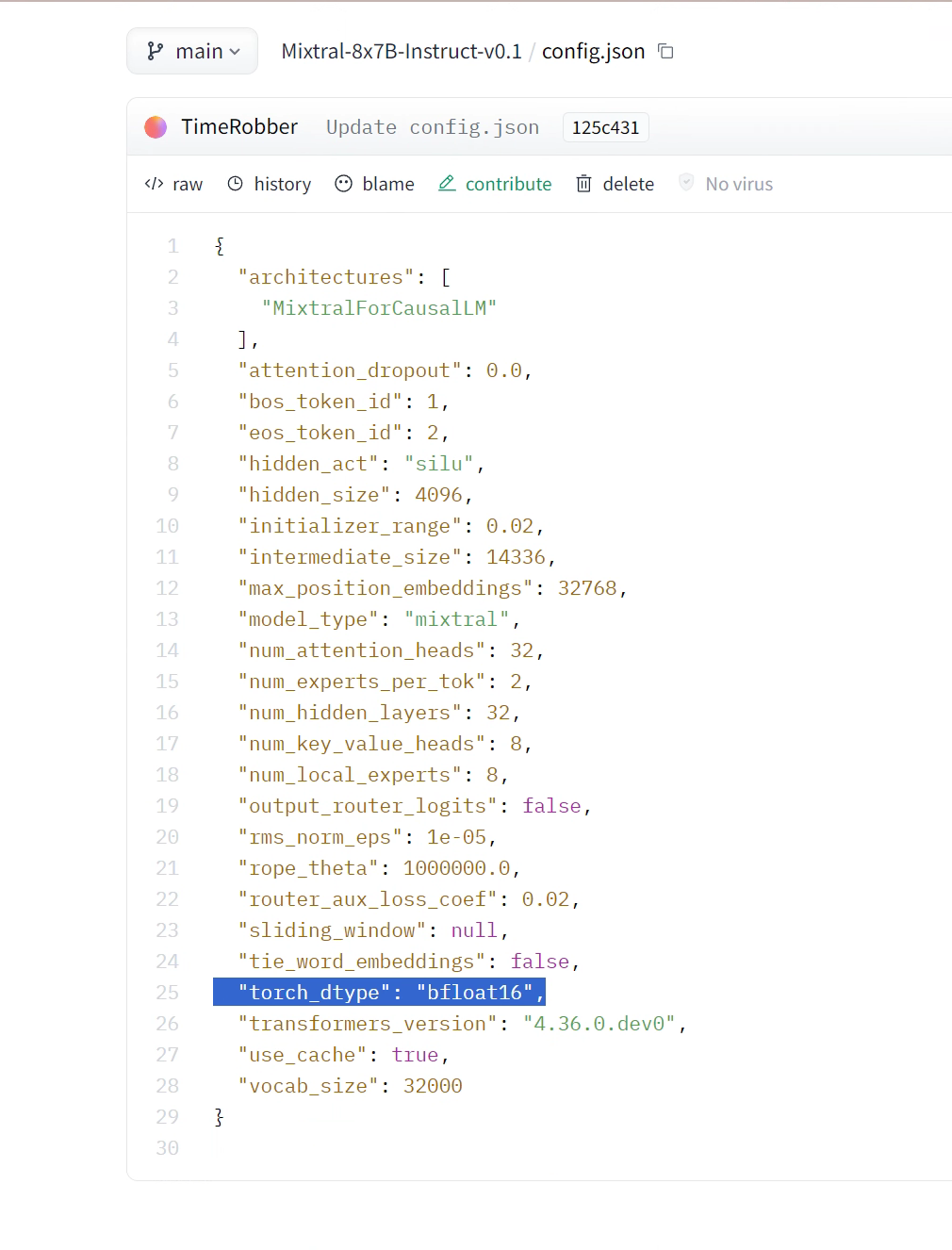
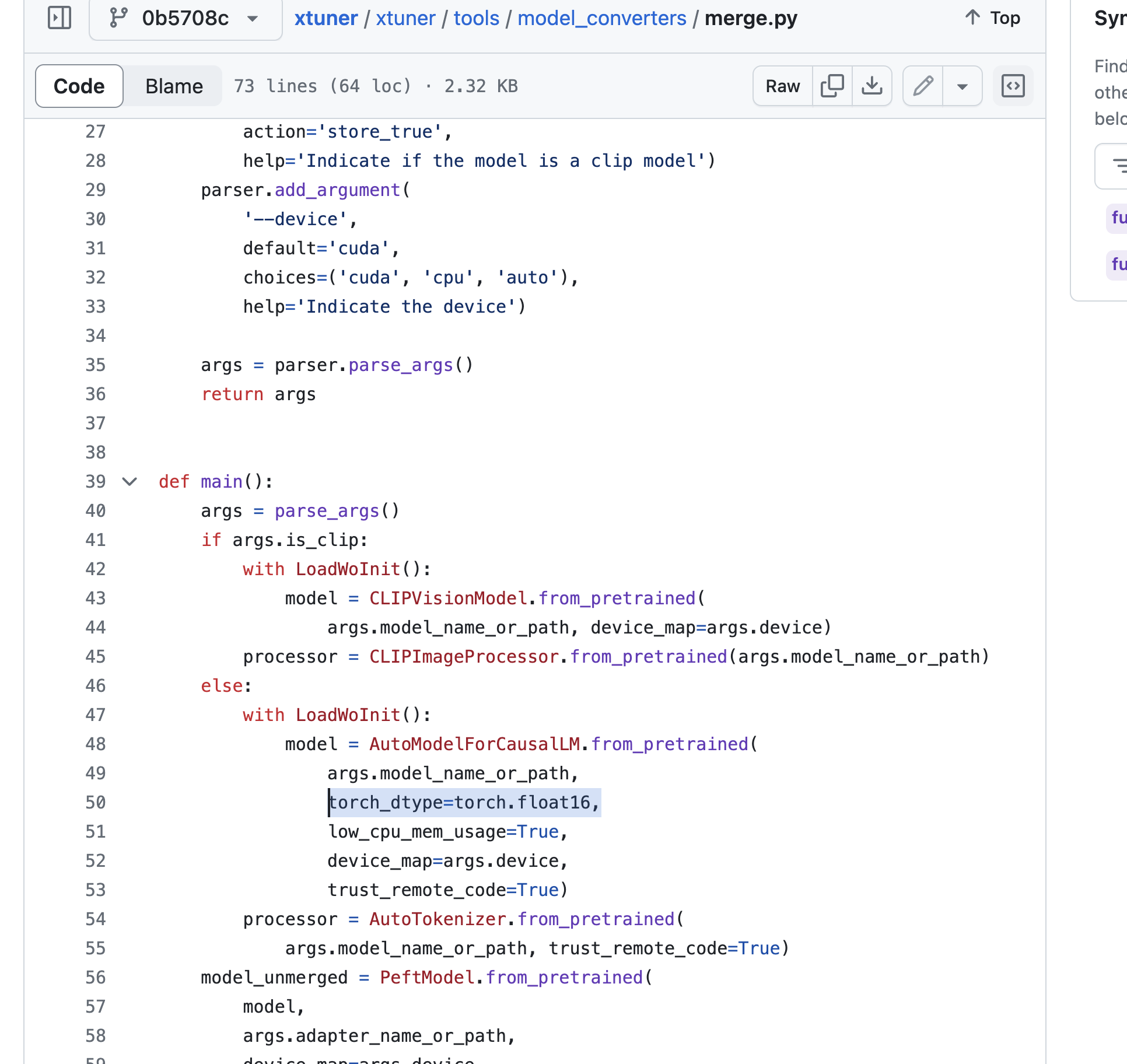
注意，xtuner默认merge出来是fp16的模型！！！！，然而mixtral原版是bf16

原因在于xtuner的merge.py默认用的float16，在v2中贾斯汀更改为了bfloat16! 这样最终模型的config.json才跟原版一致

2.4 模型的推理

2.4.1 V1/V2/V3三个版本的推理细节

由于单卡推不动，所以一开始用了2个卡的A100 80G(后来则也都统一用8张40G的A100推理)，并且也没用任何推理框架

原因：本来想用lmdeploy的，也就是书生浦语自家的，跟xtuner配套的推理框架，但是执行下面操作的时候，还是会OOM。因此采用最传统的huggingface 硬推的模式

一开始推理有严重的复读现象。会把喂进去的paper重新复述一遍，然后超过max len直接停了。后面改了prompt看起来比较正常了

当然，test 数据也要转化成xtuner要求的形式，类似上面描述的，只是没有了output，包含system和input两个键，如下

V1 使用下面代码推理：


import json
import csv
import torch
from transformers import AutoModelForCausalLM, AutoTokenizer
 
model_id = "hf_merge" #就是你刚刚xtuner convert merge之后的东西~！！！！！
tokenizer = AutoTokenizer.from_pretrained(model_id)
# model = AutoModelForCausalLM.from_pretrained(model_id, load_in_4bit=True, device_map="auto")
model = AutoModelForCausalLM.from_pretrained(model_id, torch_dtype=torch.float16, device_map="auto")
 
with open("paper_formatted_review_test.jsonl", "r", encoding='utf-8') as file:
    data = json.loads(file.read())  
 
with open("replies.csv", "w", newline="", encoding="utf-8") as csvfile:
    fieldnames = ['system', 'input', 'reply']
    writer = csv.DictWriter(csvfile, fieldnames=fieldnames)
    writer.writeheader()
 
    updated_data = []
 
    with open("log.txt", "w", encoding='utf-8') as log_file:
 
        for item in data:
            system_text = """
                You have received a batch of complete papers in the field of machine learning. As a professional reviewer, your task is to evaluate each paper based on the following four criteria: significance and innovation, possible reasons for acceptance, possible reasons for rejection, and suggestions for improvement. Please ensure that for each criterion, you summarize and provide 4 detailed supporting points from the content of the paper. The criteria you need to focus on are:
                1. Significance and Innovation: Assess the importance of the paper in its research field and the innovation of its methods or findings.
                2. Possible Reasons for Acceptance: Summarize reasons that may support the acceptance of the paper, based on its quality, research results, experimental design, etc.
                3. Possible Reasons for Rejection: Identify and explain flaws or shortcomings that could lead to the paper's rejection.
                4. Suggestions for Improvement: Provide specific suggestions to help the authors improve the paper and increase its chances of acceptance.
                After reading the content of the paper provided below, focus on the above four criteria and provide the required four detailed evaluation points for each criterion. There is no need to reply to the paper's original text; just extract and summarize information related to these criteria from the provided paper.
                complete paper content :
            """
            user_input = item["conversation"][0]["input"]
 
            out_input= """
                Based on your detailed reading and understanding of the paper, provide 4 detailed evaluation points for each of the above criteria. Your review should be based on the specific content of the paper, ensuring that each point you raise is fully supported by the content of the paper.
            """
            
            messages = [
                {"role": "user", "content": system_text + user_input + out_input},
            ]
            
            input_ids = tokenizer.apply_chat_template(messages, return_tensors="pt").to("cuda")
            outputs = model.generate(input_ids, max_new_tokens=1000)
            
            decoded_output = tokenizer.decode(outputs[0], skip_special_tokens=True)
 
            last_user_input_start = decoded_output.rfind("[INST]")
 
            if last_user_input_start != -1:
                last_user_input_end = decoded_output.find("[/INST]", last_user_input_start)
                
                if last_user_input_end != -1:
                    final_response = decoded_output[last_user_input_end + 7:].strip()
                else:
                    final_response = decoded_output[last_user_input_start:].strip()
            else:
                final_response = decoded_output
 
            print(final_response)
 
            writer.writerow({'system': system_text, 'input': user_input, 'reply': final_response})
 
            log_file.write(str({'system': system_text, 'input': user_input, 'reply': final_response}) + "\n")
 
            updated_conversation = item["conversation"] + [{"reply": final_response}]
            updated_item = {"conversation": updated_conversation}
            updated_data.append(updated_item)
 
with open("updated_conversations.json", "w", encoding='utf-8') as file:
    json.dump(updated_data, file, ensure_ascii=False, indent=4)

v2、v3使用的跟上面一样，只是改了system prompt(代码见七月大模型商用项目之审稿GPT微调实战)

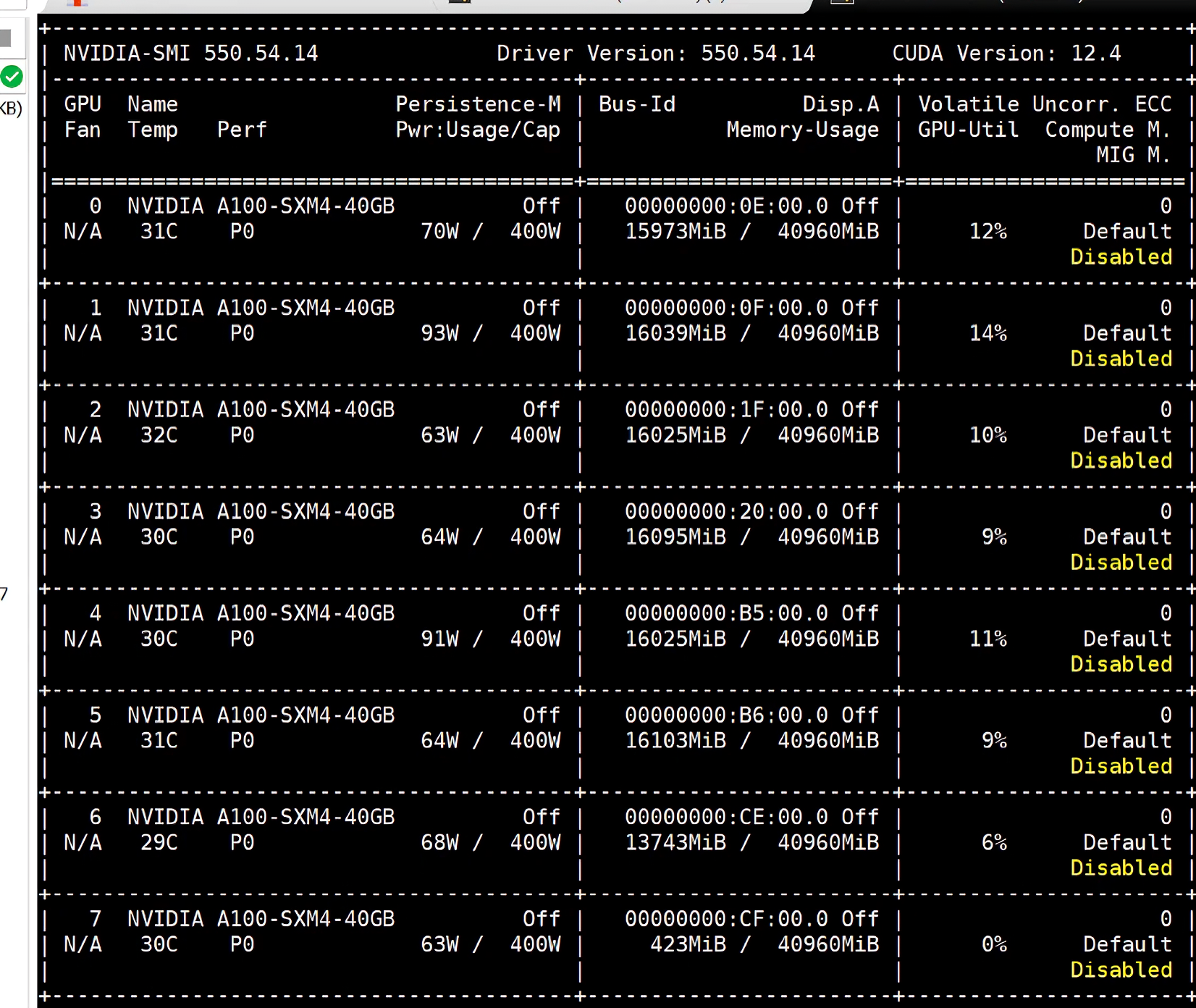
每篇文章差不多40秒推出来，8张40G A100，大概需要3小时推理285篇test data

最终，v2、v3的推理显存占用(bf16)：

2.4.2 推理中遇到的一些问题

不论是v1还是v2，loss比较难下降。好不容易v2的1.5w条数据，最终loss下降的到0.7左右：

推测原因可能是因为bs太小，但是bs调到2会爆显存，毕竟v2是lora，不是qlora、所有的target module基本都加了，且lora rank =64

v3的loss下降到0.5左右！！！然而推出来会有一些不作答的情况，可能因为prompt中设置了“示弱”，要求模型必须根据文章内容，有support才给出评论，个人认为也是好事，比瞎说要强

2.5 模型的评估：首次把对GPT4-1106的胜率达到了80%

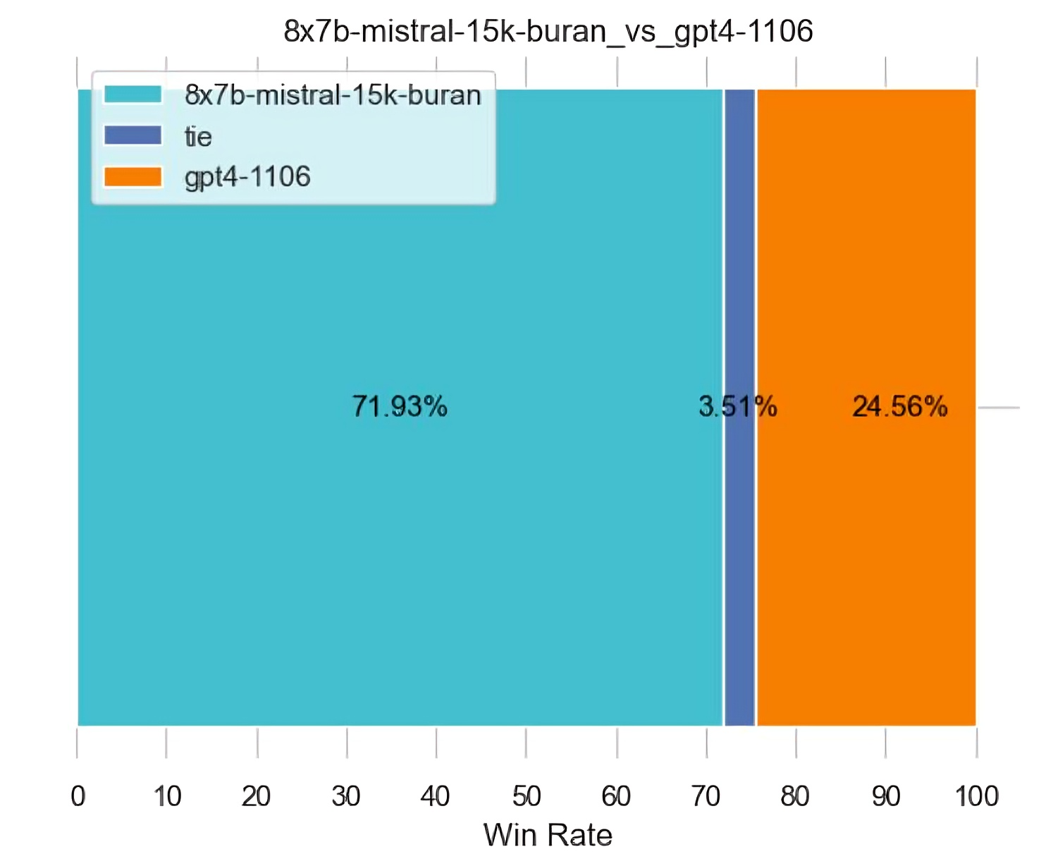
最终，在同样的测试数据集下，V2版本下的mixtral 8×7b把对GPT4-1106的胜率首次超过了80％，略胜之前微调其他模型的结果：之前llama2 7B为63.16%、llama2 13B为75.44%、gemma 7b则为之前最好结果78.95%

声明：本文内容由网友自发贡献，不代表【wpsshop博客】立场，版权归原作者所有，本站不承担相应法律责任。如您发现有侵权的内容，请联系我们。转载请注明出处：https://www.wpsshop.cn/w/小蓝xlanll/article/detail/433177

七月论文审稿GPT第4版：通过paper-review数据集微调Mixtral-8x7b，对GPT4胜率超过80%

前言

第一部分 通过llama factory微调mixtral 8x7b

1.1 模型训练：最终通过4张48G的A40跑15K数据

1.1.1 环境配置

1.1.2 训练代码：分别基于1.5K、15K数据训练

1.2 模型推理

1.2.1 部署API接口

1.2.2 调用API接口

第二部分 通过xtuner微调mixtral 8x7b

2.1 微调之前的准备：Xtuner安装、数据格式修改、数据组织、config

2.1.1 框架Xtuner的安装

2.1.2 数据格式修改

2.1.3 修改数据组织格式

2.1.4 config

2.1.5 最终config.py展示

2.2 训练细节：从5K数据微调到15K数据+qlora微调、15K数据+全量微调

2.2.1 v1：5K数据 + qlora

2.2.2 v2：15K数据 + qlora

2.2.3 v3：15K + 全量微调 + 没开量化 + 纯bf16

2.3 adapter的保存/合并

2.3.1 转化保存后的adapter

2.3.2 合并模型和adapter(仅针对v1、v2)

2.4 模型的推理

2.4.1 V1/V2/V3三个版本的推理细节

2.4.2 推理中遇到的一些问题

2.5 模型的评估：首次把对GPT4-1106的胜率达到了80%

第一部分通过llama factory微调mixtral 8x7b

第二部分通过xtuner微调mixtral 8x7b