【计算机视觉】局部图像描述子：SIFT算法_sift计算机视觉

【计算机视觉】局部图像描述子：SIFT算法

1. SIFT算法的原理

1.1 SIFT算法的目标与思想

1.1.1 算法目标

在不同的尺度空间上找特征点，这里的特征点指一些十分突出的点，不会因光照、尺度、旋转等因素的改变而消失，比如角点、边缘点、暗区域的亮点或亮区域的暗点等。最后找出两幅图像之间的特征点，并找到它们之间的匹配关系。

1.1.2 算法思想

1. 通过尺度空间和方向分配确定特征点的位置和方向，满足尺度不变性和旋转不变性

2. 对于特征点进行特征描述

3. 通过特征点的两两比较找出相互匹配的若干对特征点，建立图像之间对应关系

1.2 尺度空间的思想和表示

1.2.1 尺度空间的思想

通过对原始图像进行尺度变换，获得多尺度空间下的空间表示。从而实现边缘、角点检测和不同分辨率上的特征提取，以满足特征点的尺度不变性。

1.2.2 尺度空间的表示

由于尺度空间满足人眼从近到远逐渐模糊的成像过程，因此算法中将图像的尺度空间定义为变换尺度的高斯函数与原图像的卷积。σ指尺度空间因子，σ越大越模糊，越小越平滑，所以大尺度对应图像表观特征，小尺度对应图像细节特征。
$$\begin{gathered} 尺度空间表示：L(x,y,\sigma )=G(x,y,\sigma )\ast I(x,y) \\ 高斯函数：G(x,y,\sigma )=\frac{1}{2\pi {\sigma }^2}{e}^{-\frac{(x-m/2{)}^2+(y-n/2{)}^2}{2{\sigma }^2}} \end{gathered}$$

1.3 高斯金字塔的构建

SIFT算法中的空间特征表示采用高斯金字塔进行表示。高斯金字塔的构建步骤分为：1. 对图像进行下采样; 2. 对图像做高斯平滑。

图像下采样：将原始图像进行不断地下采样，得到一系列大小不一的图像，由大到小，由下到上构建金字塔结构。

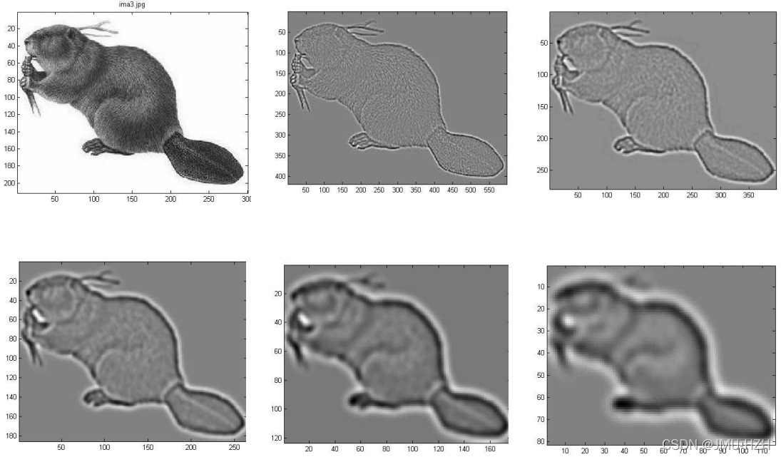
高斯平滑：为了体现尺度空间的连续性，高斯金字塔在每次下采样后，在该尺度的图像上进行多次不同尺度的高斯模糊（如上图，每个尺度的图像都会有多张越来越模糊的图像）。这里需要注意的一个小问题，每次执行下采样操作时，隔点采样的图像是每组尺度位于中间的高斯图像（假设一个尺度空间有5张越来越模糊的高斯图像，取第3张进行下采样）。

1.4 高斯差分金字塔和DOG函数

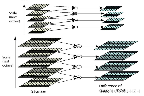
如图所示，将高斯金字塔每组中的上下两层图像进行相减就获得一系列的高斯差分图像所构成的高斯差分金字塔。(通过差值可以看出图像上像素值的变化情况)

DOG函数（Difference of Gaussian）表达式如下：
L ( x , y , σ ) = G ( x , y , σ ) ∗ I ( x , y ) D ( x , y , σ ) = [ G ( x , y , k σ ) − G ( x , y , σ ) ] ∗ I ( x , y ) = L ( x , y , k σ ) − L ( x , y , σ )

$$\begin{gathered} L(x, y, \sigma)=G(x, y, \sigma) * I(x, y) \\\\ D(x, y, \sigma)=[G(x, y, k \sigma)-G(x, y, \sigma)] * I(x, y) \\\\ =L(x, y, k \sigma)-L(x, y, \sigma) \end{gathered}$$ L(x,y,σ)=G(x,y,σ)∗I(x,y)D(x,y,σ)=[G(x,y,kσ)−G(x,y,σ)]∗I(x,y)=L(x,y,kσ)−L(x,y,σ)​

1.5 DOG局部极值检测

1.5.1 初步定位关键点

上图是高斯差分金字塔某尺度的高斯差分图像。在得到高斯金字塔后，SIFT算法对关键点进行初步筛选，筛选方法是每个尺度组中的一张高斯差分图像与相邻的两张高斯差分图像进行比较获得最后的极值点。（这里比较的高斯差分图像不能是每个尺度组的第一张图像和最后一张图像，因为这两张图像只能找到一张相邻图像。因此假设每组图像有S张高斯差分图像，但能进行筛选的高斯差分图像只有(S-2)张）

初步筛选的策略是高斯差分图像（非尺度组中的首尾图像）中的某点像素与图像域（周围的8个点）、尺度域（上下各9个点）共26个点进行比较找到极值点（27个点中差值最小的点或最大的点）作为初步关键点。

1.5.2 精确定位关键点

上述的方法通过在离散空间中（27个点进行比较）找到极值点，它与连续空间中的极值点还是有一定的偏差（如上图）。因此为了提高关键点的稳定性，我们需要对DOG函数进行拟合（这里采用泰勒展开）。
$$D(X)=D+\frac{\partial D^T}{\partial X}X+\frac{1}{2}{X}^T\frac{{\partial }^{2}D}{\partial X^2}X$$
然后对D(X)进行求导，并令其导数为0（求极值），最终获得偏移量公式：
$$\hat{X}=-\frac{{\partial }^2{D}^{-1}}{\partial X^2}\frac{\partial D}{\partial X}$$
这时候将初筛关键点的信息带入偏移量公式获得最后的实际偏移量：
$$\begin{gathered} X=(x,y,\sigma {)}^T带入偏移量公式 \\ 获得实际偏移量：\hat{X}=(x,y,\sigma {)}^T \end{gathered}$$
在实际偏移量中，如果(x, y, σ)任意一个维度的偏移量大于0.5，则认为该极值点与理想极值点有较大偏差，因此需要进行插值调整直至拟合（算法设定了一个规则，若迭代插值超过5次偏移量还大于0.5则剔除该关键点）。

1.5.3 消除边缘效应

由于DOG函数在图像边缘会产生较强的边缘响应，因此需要排除边缘响应。DoG函数的峰值点在边缘方向有较大的主曲率，而在垂直边缘的方向有较小的主曲率。算法通过该特性进行边缘效应的消除。首先可以获得特征点处的Hessian矩阵（将该点的坐标以及尺度参数信息带入DOG函数，通过泰勒展开化简可获得Hessian矩阵）
H = [ D x x D x y D x y D y y ] H=\left[

$$\begin{array}{ll} D_{x x} & D_{x y} \\ D_{x y} & D_{y y} \end{array}$$ \right] H=[Dxx​Dxy​​Dxy​Dyy​​]
Hessian矩阵的特征值表示的是在X方向和Y方向上的梯度
$$\begin{array}{rl}& \mathrm{Tr}(H)=D_{xx}+D_{yy}=\alpha +\beta \\ & \mathrm{Det}(H)=D_{xx}{D}_{yy}-{\left(D_{xy}\right)}^2=\alpha \beta \end{array}$$
通过Tr(H)和Det(H)求主曲率
$$\frac{\mathrm{Tr}(H{)}^2}{\mathrm{Det}(H)}=\frac{(a+\beta {)}^2}{a\beta }$$
通过主曲率的公式可以很容易发现，当α和β相等时曲率最小（非边缘情况下）。而当特征点位于边缘时会出现α或β中一个值大一个值小的情况，当两个方向梯度的比值越大（越趋向边缘），曲率越大。因此需要设定一个阈值，当曲率小于某个阈值时保留特征点，反之剔除。（论文中设定该阈值为1.2）
$$\frac{\mathrm{Tr}(H{)}^2}{\mathrm{Det}(H)}<T（T=1.2）$$

1.6 关键点方向分配

通过尺度不变性求极值点，可以使其具有缩放不变的性质。而利用关键点邻域像素的梯度方向分布特性，可以为每个关键点指定方向参数方向， 从而使描述子对图像旋转具有不变性。极值点的梯度表示公式如下：
$$\begin{gathered} \mathrm{grad}I(x,y)=\left(\frac{\partial I}{\partial x},\frac{\partial I}{\partial y}\right) \\ 梯度幅值：m(x,y)=\sqrt{(L(x+1,y)-L(x-1,y){)}^2+(L(x,y+1)-L(x,y-1){)}^2} \\ 梯度方向：\theta (x,y)={\tan }^{-1}\left[\frac{L(x,y+1)-L(x,y-1)}{L(x+1,y)-L(x-1,y)}\right] \end{gathered}$$
当获得准确的关键点定位后，可以通过将该点领域像素内的点进行梯度计算，获得一系列的梯度方向和幅值。

算法将方向划分为36个选择（即每10°为一个方向选择；有的代码中按每45°为一个选择，共8个选择），通过对计算出来领域像素内的点的梯度进行投票（每个梯度都求出了一个方向，求这个方向是在36个选择中的哪一个）

投票过程我们将其通过梯度直方图的方式显示。梯度直方图的峰值即为该特征点的主方向。算法中又规定了当某梯度方向的投票数大于峰值的80%，则将其定义为关键点的辅方向，通过将主方向和辅方向进行插值拟合可以获得更稳定和准确的方向。（仅有15%的点被赋予多个方向，因此该操作的复杂度尚可接受）

综上，可以检测出含有尺度、方向、位置的SIFT特征点。

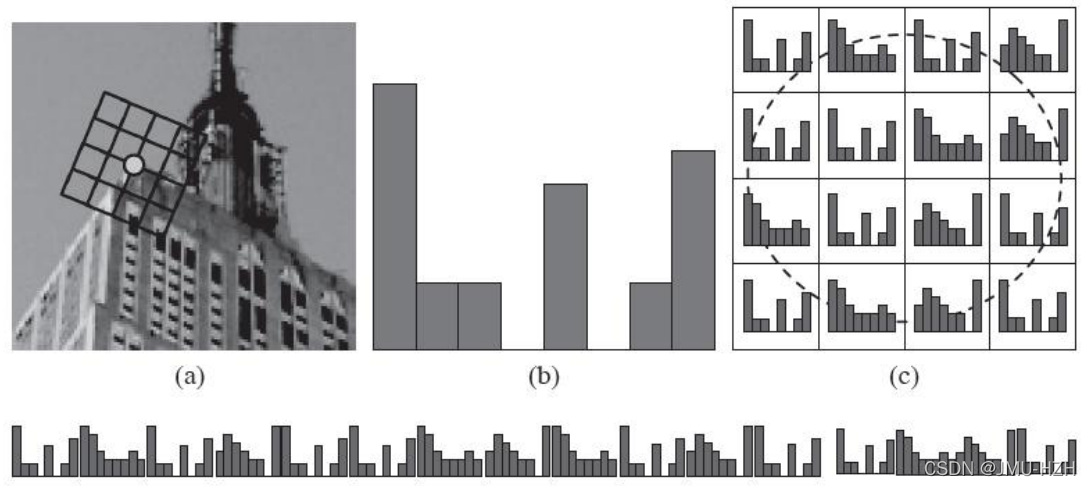
1.7 SIFT特征点描述

当获得特征点位置、尺度、方向后，需要构建一个对于该特征点的特征描述，用一组向量将该特征点表示出来并且不受光照和视角变化的影响。

构建过程：
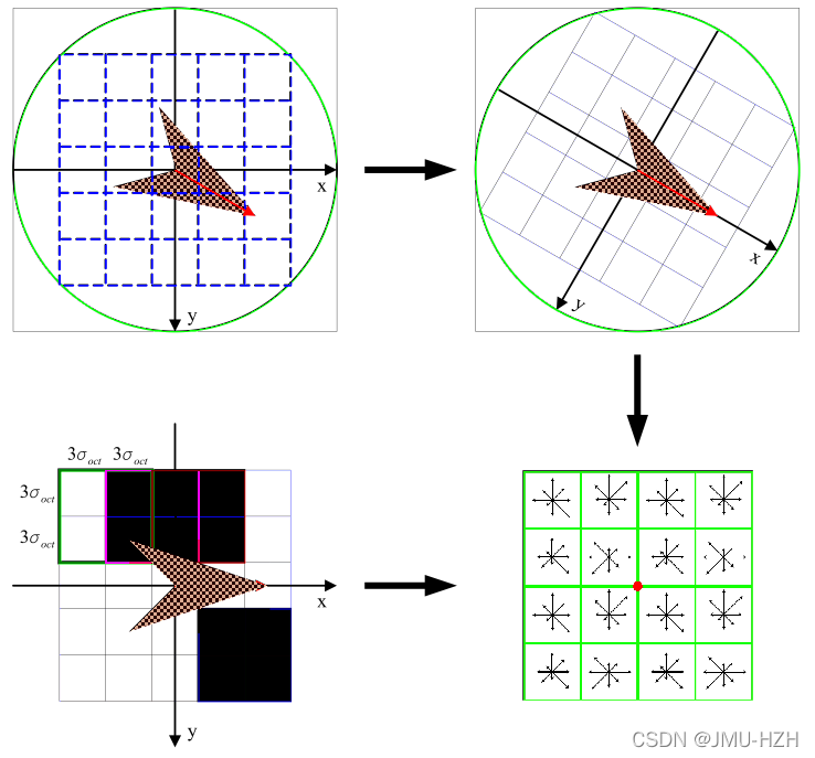
1. 计算特征点周围领域像素的特征信息，对其进行梯度求解。例如：一个4x4的窗口内分别计算每个1x1窗口朝八个方向的幅度（东南西北、东南、东北、西南、西北），因此将构成一个4x4x8的128维向量。（综合效果最佳）
2. 将计算出来的特征点领域像素梯度转到所在方向（特征点方向），这个过程通过插值的方法，相当于将图像的像素进行了一定程度的旋转（旋转后像素坐标改变）
1
2
3

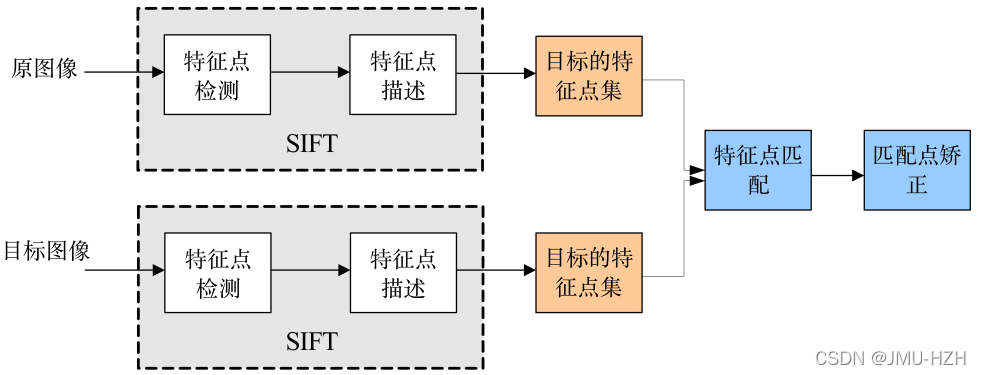
1.8 关键点匹配

算法通过对两张图片（原图和模板图）建立关键点描述子集合。目标的识别是通过两点集内关键点描述子的比对来完成。具有128维的关键点描述子的相似性度量采用欧式距离。
$$\begin{gathered} 模板图中关键点描述子:R_i=\left(r_{i1},r_{i2},\cdots ,r_{i128}\right) \\ 实时图中关键点描述子:S_i=\left(s_{i1},s_{i2},\cdots ,s_{i128}\right) \\ 任意两描述子相似性度量:d\left(R_i,S_i\right)=\sqrt{\sum _{j=1}^{128}{\left(r_{ij}-S_{ij}\right)}^2} \\ 匹配条件：d\left(R_i,S_i\right)<Threshold \end{gathered}$$
关键点的匹配可以采用穷举法来完成，但是这样耗费的时间太多，一般都采用kd树的数据结构来完成搜索。搜索的内容是以目标图像的关键点为基准，搜索与目标图像的特征点最邻近的原图像特征点和次邻近的原图像特征点。

2. SIFT算法代码实现

这里采用VLFeat中的开源库进行SIFT特征点的提取和描述子的构建，因此在使用该代码前需下载VLFeat并将其添加至环境变量中。

# -*- coding: utf-8 -*-
from PIL import Image
from pylab import *
from numpy import *
import os
from tqdm import tqdm

# 处理图片，通过VLFeat中的开源库进行Sift特征点的检测
# imagename: 输入图片路径
# resultname: 输出检测结果（通过文本类型进行保存）
# params: 命令参数
def process_image(imagename, resultname, params="--edge-thresh 30 --peak-thresh 15"):
    if imagename[-3:] != 'pgm':
        #创建一个pgm文件
        im = Image.open(imagename).convert('L')
        im.save('D:/desktop/cv_task/sift/tmp.pgm')
        imagename ='D:/desktop/cv_task/sift/tmp.pgm'
    cmmd = str("sift "+imagename+" --output="+resultname+" "+params)

    # 通过终端进行命令行操作
    os.system(cmmd)
    print('processed', imagename, 'to', resultname)

# 读取生成的文本文件内容
def read_features_from_file(filename):
    f = loadtxt(filename)
    # 返回特征位置和描述子
    return f[:,:4], f[:,4:]

def write_featrues_to_file(filename, locs, desc):
    # 将特征位置返回到文本中
    savetxt(filename, hstack((locs,desc)))


def plot_features(im, locs, circle=False):

    def draw_circle(c,r):
        t = arange(0,1.01,.01)*2*pi
        x = r*cos(t) + c[0]
        y = r*sin(t) + c[1]
        plot(x, y, 'b', linewidth=2)

    imshow(im)
    if circle:
        for p in locs:
            draw_circle(p[:2], p[2])
    else:
        plot(locs[:,0], locs[:,1], 'ob')
    axis('off')

def match(desc1, desc2):
    desc1 = array([d/linalg.norm(d) for d in desc1])
    desc2 = array([d/linalg.norm(d) for d in desc2])

    dist_ratio = 0.6
    desc1_size = desc1.shape
    matchscores = zeros((desc1_size[0],1),'int')
    desc2t = desc2.T #预先计算矩阵转置
    for i in tqdm(range(desc1_size[0])):
        dotprods = dot(desc1[i,:],desc2t) #向量点乘
        dotprods = 0.9999*dotprods
        # 反余弦和反排序，返回第二幅图像中特征的索引
        indx = argsort(arccos(dotprods))

        #检查最近邻的角度是否小于dist_ratio乘以第二近邻的角度
        if arccos(dotprods)[indx[0]] < dist_ratio * arccos(dotprods)[indx[1]]:
            matchscores[i] = int(indx[0])

    return matchscores

def match_twosided(desc1, desc2):
    matches_12 = match(desc1, desc2)
    matches_21 = match(desc2, desc1)

    ndx_12 = matches_12.nonzero()[0]

    # 去除不对称的匹配
    for n in ndx_12:
        if matches_21[int(matches_12[n])] != n:
            matches_12[n] = 0

    return matches_12

def appendimages(im1, im2):
    rows1 = im1.shape[0]
    rows2 = im2.shape[0]

    if rows1 < rows2:
        im1 = concatenate((im1, zeros((rows2-rows1,im1.shape[1]))),axis=0)
    elif rows1 >rows2:
        im2 = concatenate((im2, zeros((rows1-rows2,im2.shape[1]))),axis=0)
    return concatenate((im1,im2), axis=1)

def plot_matches(im1,im2,locs1,locs2,matchscores,show_below=False):
    im3=appendimages(im1,im2)
    if show_below:
        im3=vstack((im3,im3))
    imshow(im3)

    cols1 = im1.shape[1]
    for i in range(len(matchscores)):
        if matchscores[i]>0:
            plot([locs1[i,0],locs2[matchscores[i,0],0]+cols1], [locs1[i,1],locs2[matchscores[i,0],1]],'c')
    axis('off')


if "__main__" == __name__:
    img1 = 'D:/desktop/cv_task/sift/test4.jpg'
    img2 = 'D:/desktop/cv_task/sift/test5.jpg'
    im1 = array(Image.open(img1))
    im2 = array(Image.open(img2))

    #process_image(im1f, 'D:/desktop/cv_task/sift/out_sift_1.txt')
    l1,d1 = read_features_from_file('D:/desktop/cv_task/sift/out_sift_1.txt')

    #process_image(im2f, 'D:/desktop/cv_task/sift/out_sift_2.txt')
    l2,d2 = read_features_from_file('D:/desktop/cv_task/sift/out_sift_2.txt')

    matches = match_twosided(d1, d2)
    figure()
    gray()
    plot_matches(im1,im2,l1,l2,matches)
    show()
1
2
3
4
5
6
7
8
9
10
11
12
13
14
15
16
17
18
19
20
21
22
23
24
25
26
27
28
29
30
31
32
33
34
35
36
37
38
39
40
41
42
43
44
45
46
47
48
49
50
51
52
53
54
55
56
57
58
59
60
61
62
63
64
65
66
67
68
69
70
71
72
73
74
75
76
77
78
79
80
81
82
83
84
85
86
87
88
89
90
91
92
93
94
95
96
97
98
99
100
101
102
103
104
105
106
107
108
109
110
111
112
113
114
115
116
117
118
119
120
121
122
123

opencv代码：

import cv2
import matplotlib.pyplot as plt

img1 = cv2.imread('sift/test1.jpg')
gray1 = cv2.cvtColor(img1, cv2.COLOR_BGR2GRAY)
sift = cv2.xfeatures2d.SIFT_create()
keypoints_1, descriptors_1 = sift.detectAndCompute(img1,None)
img_1 = cv2.drawKeypoints(gray1,keypoints_1,img1)
plt.imshow(img_1)
plt.show()
plt.imsave("save.jpg",img_1)
1
2
3
4
5
6
7
8
9
10
11

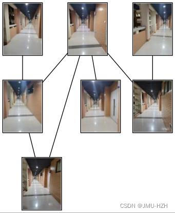
3. 匹配地理标记图像

地理标记图像是基于SIFT特征匹配完成的，大体思想就是将一系列的图像进行一一对应匹配，若特征点匹配对大于设置的阈值（代码中设置为2）则判断两个地理图像是有联系的，将其进行连接。

代码执行环境：
1. 安装Graphviz(https://www.graphviz.org/download/)，下载文件库，并将其bin文件添加到电脑的环境变量中。
2. pip install graphviz
3. pip insyall pydot
4. pip install pydot-ng

若出现FileNotFoundError: [WinError 2] "dot" not found in path.
解决方案：找到anaconda/lib/site-package下的pydot.py，将里面的self.prog = 'dot'改为self.prog = 'dot.exe'可解决。
1
2
3
4
5
6
7
8

# -*- coding: utf-8 -*-
from pylab import *
from PIL import Image
#from PCV.localdescriptors import sift
from PCV.tools import imtools
import pydot
from tqdm import tqdm
import os
import numba as nb
nb.jit

def process_image(imagename, resultname, params="--edge-thresh 40 --peak-thresh 20"):
    if imagename[-3:] != 'pgm':
        #创建一个pgm文件
        im = Image.open(imagename).convert('L')
        im.save('tmp.pgm')
        imagename ='tmp.pgm'
    cmmd = str("sift "+imagename+" --output="+resultname+" "+params)

    # 通过终端进行命令行操作
    os.system(cmmd)
    print('processed', imagename, 'to', resultname)

# 读取生成的文本文件内容
def read_features_from_file(filename):
    f = loadtxt(filename)
    # 返回特征位置和描述子
    return f[:,:4], f[:,4:]

def match(desc1, desc2):
    desc1 = array([d/linalg.norm(d) for d in desc1])
    desc2 = array([d/linalg.norm(d) for d in desc2])

    dist_ratio = 0.6
    desc1_size = desc1.shape
    matchscores = zeros((desc1_size[0],1),'int')
    desc2t = desc2.T #预先计算矩阵转置
    for i in tqdm(range(desc1_size[0])):
        dotprods = dot(desc1[i,:],desc2t) #向量点乘
        dotprods = 0.9999*dotprods
        # 反余弦和反排序，返回第二幅图像中特征的索引
        indx = argsort(arccos(dotprods))

        #检查最近邻的角度是否小于dist_ratio乘以第二近邻的角度
        if arccos(dotprods)[indx[0]] < dist_ratio * arccos(dotprods)[indx[1]]:
            matchscores[i] = int(indx[0])

    return matchscores

def match_twosided(desc1, desc2):
    matches_12 = match(desc1, desc2)
    matches_21 = match(desc2, desc1)

    ndx_12 = matches_12.nonzero()[0]

    # 去除不对称的匹配
    for n in ndx_12:
        if matches_21[int(matches_12[n])] != n:
            matches_12[n] = 0

    return matches_12

if "__main__" == __name__:
    download_path = "D:/desktop/cv_task/photo"
    path = "D:/desktop/cv_task/photo"

    imlist = imtools.get_imlist(download_path)
    nbr_images = len(imlist)

    featlist = [imname[:-3] + 'sift' for imname in imlist]

    for i, imname in enumerate(imlist):
        process_image(imname, featlist[i])

    matchscores = zeros((nbr_images, nbr_images))

    for i in tqdm(range(nbr_images)):
        for j in range(i, nbr_images):  # only compute upper triangle
            print('comparing ', imlist[i], imlist[j])
            l1, d1 = read_features_from_file(featlist[i])
            l2, d2 = read_features_from_file(featlist[j])
            matches = match_twosided(d1, d2)
            nbr_matches = sum(matches > 0)
            print('number of matches = ', nbr_matches)
            matchscores[i, j] = nbr_matches

    # copy values
    for i in range(nbr_images):
        for j in range(i + 1, nbr_images):  # no need to copy diagonal
            matchscores[j, i] = matchscores[i, j]

    # 可视化

    threshold = 2  # min number of matches needed to create link

    g = pydot.Dot(graph_type='graph')  # don't want the default directed graph

    for i in range(nbr_images):
        for j in range(i + 1, nbr_images):
            if matchscores[i, j] > threshold:
                # first image in pair
                im = Image.open(imlist[i])
                im.thumbnail((100, 100))
                filename = path + str(i) + '.jpg'
                im.save(filename)  # need temporary files of the right size
                g.add_node(pydot.Node(str(i), fontcolor='transparent', shape='rectangle', image=filename))

                # second image in pair
                im = Image.open(imlist[j])
                im.thumbnail((100, 100))
                filename = path + str(j) + '.jpg'
                im.save(filename)  # need temporary files of the right size
                g.add_node(pydot.Node(str(j), fontcolor='transparent', shape='rectangle', image=filename))

                g.add_edge(pydot.Edge(str(i), str(j)))

    g.write_jpg('result.jpg')
1
2
3
4
5
6
7
8
9
10
11
12
13
14
15
16
17
18
19
20
21
22
23
24
25
26
27
28
29
30
31
32
33
34
35
36
37
38
39
40
41
42
43
44
45
46
47
48
49
50
51
52
53
54
55
56
57
58
59
60
61
62
63
64
65
66
67
68
69
70
71
72
73
74
75
76
77
78
79
80
81
82
83
84
85
86
87
88
89
90
91
92
93
94
95
96
97
98
99
100
101
102
103
104
105
106
107
108
109
110
111
112
113
114
115
116
117