目标检测详解

---

前言

提示：这里是本文要记录的大概内容：
图像中若有多个我们感兴趣的目标，我们不仅想知道他们的类别，还想知道他们的具体位置，称为目标检测。

---

提示：以下是本篇文章正文内容

一、基本概念

上面我们已经知道目标检测，需要完成两项任务，即分类和定位。

目标检测的思路

想要知道某个位置存在物体，主要靠“猜”，即通过滑窗的方式，将各种可能的区域列举出来。对每一个区域就行判别，最终得到类别和坐标的信息。

边界框

在目标检测中，我们通常使用边界框来描述对象的空间位置。边界框是矩形的，由矩形左上⻆的以及右下⻆的x和y坐标决定。另⼀种常⽤的边界框表⽰⽅法是边界框中⼼的(x, y)轴坐标以及框的宽度和⾼度。
在这⾥，我们定义在这两种表⽰法之间进⾏转换的函数：

def box_corner_to_center(boxes):
	"""从（左上，右下）转换到（中间，宽度，⾼度）"""
	x1, y1, x2, y2 = boxes[:, 0], boxes[:, 1], boxes[:, 2], boxes[:, 3]
	cx = (x1 + x2) / 2
	cy = (y1 + y2) / 2
	w = x2 - x1
	h = y2 - y1
	boxes = torch.stack((cx, cy, w, h), axis=-1)
	return boxes
def box_center_to_corner(boxes):
	"""从（中间，宽度，⾼度）转换到（左上，右下）"""
	cx, cy, w, h = boxes[:, 0], boxes[:, 1], boxes[:, 2], boxes[:, 3]
	x1 = cx - 0.5 * w
	y1 = cy - 0.5 * h
	x2 = cx + 0.5 * w
	y2 = cy + 0.5 * h
	boxes = torch.stack((x1, y1, x2, y2), axis=-1)
	return boxes
# 注：图像中坐标的原点是图像的左上⻆，向右的⽅向为x轴的正⽅向，向下的⽅向为y轴的正⽅向。
# 将边界框在图中画出，以检查其是否准确。定义一个辅助函数bbox_to_rect
def bbox_to_rect(bbox, color):
	# 将边界框(左上x,左上y,右下x,右下y)格式转换成matplotlib格式：
	# ((左上x,左上y),宽,⾼)
	return plt.Rectangle(
	xy=(bbox[0], bbox[1]), width=bbox[2]-bbox[0], height=bbox[3]-bbox[1],
	fill=False, edgecolor=color, linewidth=2)
# 例：
fig = plt.imshow(img)  # 获取流对象
fig.axes.add_patch(bbox_to_rect(dog_bbox, 'blue'))
fig.axes.add_patch(bbox_to_rect(cat_bbox, 'red'));
1
2
3
4
5
6
7
8
9
10
11
12
13
14
15
16
17
18
19
20
21
22
23
24
25
26
27
28
29
30

锚框

⽬标检测算法通常会在输⼊图像中采样⼤量的区域，然后判断这些区域中是否包含我们感兴趣的⽬标，并调整区域边界从⽽更准确地预测⽬标的真实边界框（ground-truth bounding box）。
以每个像素为中⼼，⽣成多个缩放⽐和宽⾼⽐（aspect ratio）不同的边界框。

"""
假设输⼊图像的⾼度为h，宽度为w。我们以图像的每个像素为中⼼⽣成不同形状的锚框：缩放⽐为s ∈ (0, 1]，
宽⾼⽐为r > 0。那么锚框的宽度和⾼度分别是ws*sqrt(r)和hs/sqrt(r)。请注意，当中⼼位置给定时，已知宽和⾼的锚框是确定的。为了减少复杂度，我们只考虑包含取值最小的缩放比和宽高比最小的组合：
"""
def multibox_prior(data, sizes, ratios):
	"""⽣成以每个像素为中⼼具有不同形状的锚框
	data形状为：n * c * h * w
	"""
	in_height, in_width = data.shape[-2:]
	device, num_sizes, num_ratios = data.device, len(sizes), len(ratios)
	boxes_per_pixel = (num_sizes + num_ratios - 1)
	size_tensor = torch.tensor(sizes, device=device)
	ratio_tensor = torch.tensor(ratios, device=device)
	# 为了将锚点移动到像素的中⼼，需要设置偏移量。
	# 因为⼀个像素的的⾼为1且宽为1，我们选择偏移我们的中⼼0.5
	offset_h, offset_w = 0.5, 0.5
	steps_h = 1.0 / in_height # 在y轴上缩放步⻓
	steps_w = 1.0 / in_width # 在x轴上缩放步⻓
	# ⽣成锚框的所有中⼼点
	center_h = (torch.arange(in_height, device=device) + offset_h) * steps_h
	center_w = (torch.arange(in_width, device=device) + offset_w) * steps_w
	shift_y, shift_x = torch.meshgrid(center_h, center_w)
	shift_y, shift_x = shift_y.reshape(-1), shift_x.reshape(-1)
	# ⽣成“boxes_per_pixel”个⾼和宽，
	# 之后⽤于创建锚框的四⻆坐标(xmin,xmax,ymin,ymax)
	w = torch.cat((size_tensor * torch.sqrt(ratio_tensor[0]),
	sizes[0] * torch.sqrt(ratio_tensor[1:])))\
	* in_height / in_width # 处理矩形输⼊
	h = torch.cat((size_tensor / torch.sqrt(ratio_tensor[0]),
	sizes[0] / torch.sqrt(ratio_tensor[1:])))
	# 除以2来获得半⾼和半宽
	anchor_manipulations = torch.stack((-w, -h, w, h)).T.repeat(
	in_height * in_width, 1) / 2
	# 每个中⼼点都将有“boxes_per_pixel”个锚框，
	# 所以⽣成含所有锚框中⼼的⽹格，重复了“boxes_per_pixel”次
	out_grid = torch.stack([shift_x, shift_y, shift_x, shift_y],
	dim=1).repeat_interleave(boxes_per_pixel, dim=0)
	output = out_grid + anchor_manipulations
	return output.unsqueeze(0)
1
2
3
4
5
6
7
8
9
10
11
12
13
14
15
16
17
18
19
20
21
22
23
24
25
26
27
28
29
30
31
32
33
34
35
36
37
38
39
'
运行
运行

为了显⽰以图像中以某个像素为中⼼的所有锚框，我们定义了下⾯的show_bboxes函数来在图像上绘制多个边界框。

def show_bboxes(axes, bboxes, labels=None, colors=None):
	"""显⽰所有边界框"""
	def _make_list(obj, default_values=None):
	if obj is None:
	obj = default_values
	elif not isinstance(obj, (list, tuple)):
	obj = [obj]
	return obj
	labels = _make_list(labels)
	colors = _make_list(colors, ['b', 'g', 'r', 'm', 'c'])
	for i, bbox in enumerate(bboxes):
	color = colors[i % len(colors)]
	rect = bbox_to_rect(bbox.detach().numpy(), color)
	axes.add_patch(rect)
	if labels and len(labels) > i:
	text_color = 'k' if color == 'w' else 'w'
	axes.text(rect.xy[0], rect.xy[1], labels[i],
	va='center', ha='center', fontsize=9, color=text_color,
	bbox=dict(facecolor=color, lw=0))
1
2
3
4
5
6
7
8
9
10
11
12
13
14
15
16
17
18
19

交并比（loU）

杰卡德系数（Jaccard）可以衡量两组之间的相似性。给定集合A和B，他们的杰卡德系数是他们交集的⼤⼩除以他们并集的⼤⼩。对于两个边界框，我们通常将它们的杰卡德系数称为交并比（intersection over union，IoU），即两个边界框相交⾯积与相并⾯积之⽐，如下图所⽰。交并⽐的取值范围在0和1之间：0表⽰两个边界框⽆重合像素，1表⽰两个边界框完全重合。

def box_iou(boxes1, boxes2):
	"""计算两个锚框或边界框列表中成对的交并⽐"""
	box_area = lambda boxes: ((boxes[:, 2] - boxes[:, 0]) * (boxes[:, 3] - boxes[:, 1]))
	# boxes1,boxes2,areas1,areas2的形状:
	# boxes1：(boxes1的数量,4),
	# boxes2：(boxes2的数量,4),
	# areas1：(boxes1的数量,),
	# areas2：(boxes2的数量,)
	areas1 = box_area(boxes1)
	areas2 = box_area(boxes2)
	# inter_upperlefts,inter_lowerrights,inters的形状:
	# (boxes1的数量,boxes2的数量,2)
	inter_upperlefts = torch.max(boxes1[:, None, :2], boxes2[:, :2])
	inter_lowerrights = torch.min(boxes1[:, None, 2:], boxes2[:, 2:])
	inters = (inter_lowerrights - inter_upperlefts).clamp(min=0)
	# inter_areasandunion_areas的形状:(boxes1的数量,boxes2的数量)
	inter_areas = inters[:, :, 0] * inters[:, :, 1]
	union_areas = areas1[:, None] + areas2 - inter_areas
	return inter_areas / union_areas
1
2
3
4
5
6
7
8
9
10
11
12
13
14
15
16
17
18
19
'
运行
运行

标注锚框

在预测时，我们为每个图像⽣成多个锚框，预测所有锚框的类别和偏移量，根据预测的偏移量调整它们的位置以获得预测的边界框，最后只输出符合特定条件的预测边界框。

在训练数据中标注锚框

将真实边界框分配给锚框

def assign_anchor_to_bbox(ground_truth, anchors, device, iou_threshold=0.5):
	"""将最接近的真实边界框分配给锚框"""
	num_anchors, num_gt_boxes = anchors.shape[0], ground_truth.shape[0]
	# 位于第i⾏和第j列的元素x_ij是锚框i和真实边界框j的IoU
	jaccard = box_iou(anchors, ground_truth)
	# 对于每个锚框，分配的真实边界框的张量
	anchors_bbox_map = torch.full((num_anchors,), -1, dtype=torch.long,
	device=device)
	# 根据阈值，决定是否分配真实边界框
	max_ious, indices = torch.max(jaccard, dim=1)
	anc_i = torch.nonzero(max_ious >= 0.5).reshape(-1)
	box_j = indices[max_ious >= 0.5]
	anchors_bbox_map[anc_i] = box_j
	col_discard = torch.full((num_anchors,), -1)
	row_discard = torch.full((num_gt_boxes,), -1)
	for _ in range(num_gt_boxes):
		max_idx = torch.argmax(jaccard)
		box_idx = (max_idx % num_gt_boxes).long()
		anc_idx = (max_idx / num_gt_boxes).long()
		anchors_bbox_map[anc_idx] = box_idx
		jaccard[:, box_idx] = col_discard
		jaccard[anc_idx, :] = row_discard
	return anchors_bbox_map
1
2
3
4
5
6
7
8
9
10
11
12
13
14
15
16
17
18
19
20
21
22
23
'
运行
运行

标记类别和偏移量

假设⼀个锚框A被分配了⼀个真实边界框B。⼀⽅⾯，锚框A的类别将被标记为与B相同。另⼀⽅⾯，锚框A的偏移量将根据B和A中⼼坐标的相对位置以及这两个框的相对⼤⼩进⾏标记。鉴于数据集内不同的框的位置和⼤⼩不同，我们可以对那些相对位置和⼤⼩应⽤变换，使其获得分布更均匀且易于拟合的偏移量。

def offset_boxes(anchors, assigned_bb, eps=1e-6):
	"""对锚框偏移量的转换"""
	c_anc = box_corner_to_center(anchors)
	c_assigned_bb = box_corner_to_center(assigned_bb)
	offset_xy = 10 * (c_assigned_bb[:, :2] - c_anc[:, :2]) / c_anc[:, 2:]
	offset_wh = 5 * torch.log(eps + c_assigned_bb[:, 2:] / c_anc[:, 2:])
	offset = torch.cat([offset_xy, offset_wh], axis=1)
	return offset
1
2
3
4
5
6
7
8
'
运行
运行

我们使⽤真实边界框（labels参数）实现以下multibox_target函数，来标记锚框的类别和偏移量（anchors参数）。此函数将背景类别的索引设置为零，然后将新类别的整数索引递增⼀。

def multibox_target(anchors, labels):
	"""使⽤真实边界框标记锚框"""
	batch_size, anchors = labels.shape[0], anchors.squeeze(0)
	batch_offset, batch_mask, batch_class_labels = [], [], []
	device, num_anchors = anchors.device, anchors.shape[0]
	for i in range(batch_size):
		label = labels[i, :, :]
		anchors_bbox_map = assign_anchor_to_bbox(
		label[:, 1:], anchors, device)
		bbox_mask = ((anchors_bbox_map >= 0).float().unsqueeze(-1)).repeat(
		1, 4)
		# 将类标签和分配的边界框坐标初始化为零
		class_labels = torch.zeros(num_anchors, dtype=torch.long,
		device=device)
		assigned_bb = torch.zeros((num_anchors, 4), dtype=torch.float32,
		device=device)
		# 使⽤真实边界框来标记锚框的类别。
		# 如果⼀个锚框没有被分配，我们标记其为背景（值为零）
		indices_true = torch.nonzero(anchors_bbox_map >= 0)
		bb_idx = anchors_bbox_map[indices_true]
		class_labels[indices_true] = label[bb_idx, 0].long() + 1
		assigned_bb[indices_true] = label[bb_idx, 1:]
		# 偏移量转换
		offset = offset_boxes(anchors, assigned_bb) * bbox_mask
		batch_offset.append(offset.reshape(-1))
		batch_mask.append(bbox_mask.reshape(-1))
		batch_class_labels.append(class_labels)
	bbox_offset = torch.stack(batch_offset)
	bbox_mask = torch.stack(batch_mask)
	class_labels = torch.stack(batch_class_labels)
	return (bbox_offset, bbox_mask, class_labels)
1
2
3
4
5
6
7
8
9
10
11
12
13
14
15
16
17
18
19
20
21
22
23
24
25
26
27
28
29
30
31
'
运行
运行

使用非极大值抑制预测边界框

在预测时，我们先为图像⽣成多个锚框，再为这些锚框⼀⼀预测类别和偏移量。下⾯我们实现了offset_inverse函数，该函数将锚框和偏移量预测作为输⼊，并应⽤逆偏移变换来返回预测的边界框坐标。

def offset_inverse(anchors, offset_preds):
	"""根据带有预测偏移量的锚框来预测边界框"""
	anc = box_corner_to_center(anchors)
	pred_bbox_xy = (offset_preds[:, :2] * anc[:, 2:] / 10) + anc[:, :2]
	pred_bbox_wh = torch.exp(offset_preds[:, 2:] / 5) * anc[:, 2:]
	pred_bbox = torch.cat((pred_bbox_xy, pred_bbox_wh), axis=1)
	predicted_bbox = box_center_to_corner(pred_bbox)
	return predicted_bbox
1
2
3
4
5
6
7
8
'
运行
运行

当有许多锚框时，可能会输出许多相似的具有明显重叠的预测边界框，都围绕着同⼀⽬标。为了简化输出，我们可以使⽤⾮极⼤值抑制（non-maximum suppression，NMS）合并属于同⼀⽬标的类似的预测边界框。
以下nms函数按降序对置信度进⾏排序并返回其索引。

def nms(boxes, scores, iou_threshold):
	"""对预测边界框的置信度进⾏排序"""
	B = torch.argsort(scores, dim=-1, descending=True)
	keep = [] # 保留预测边界框的指标
	while B.numel() > 0:
		i = B[0]
		keep.append(i)
		if B.numel() == 1: break
		iou = box_iou(boxes[i, :].reshape(-1, 4),
		boxes[B[1:], :].reshape(-1, 4)).reshape(-1)
		inds = torch.nonzero(iou <= iou_threshold).reshape(-1)
		B = B[inds + 1]
	return torch.tensor(keep, device=boxes.device)
1
2
3
4
5
6
7
8
9
10
11
12
13
'
运行
运行

定义以下multibox_detection函数来将⾮极⼤值抑制应⽤于预测边界框。

def multibox_detection(cls_probs, offset_preds, anchors, nms_threshold=0.5, pos_threshold=0.009999999):
	"""使⽤⾮极⼤值抑制来预测边界框"""
	device, batch_size = cls_probs.device, cls_probs.shape[0]
	anchors = anchors.squeeze(0)
	num_classes, num_anchors = cls_probs.shape[1], cls_probs.shape[2]
	out = []
	for i in range(batch_size):
		cls_prob, offset_pred = cls_probs[i], offset_preds[i].reshape(-1, 4)
		conf, class_id = torch.max(cls_prob[1:], 0)
		predicted_bb = offset_inverse(anchors, offset_pred)
		keep = nms(predicted_bb, conf, nms_threshold)
		# 找到所有的non_keep索引，并将类设置为背景
		all_idx = torch.arange(num_anchors, dtype=torch.long, device=device)
		combined = torch.cat((keep, all_idx))
		uniques, counts = combined.unique(return_counts=True)
		non_keep = uniques[counts == 1]
		all_id_sorted = torch.cat((keep, non_keep))
		class_id[non_keep] = -1
		class_id = class_id[all_id_sorted]
		conf, predicted_bb = conf[all_id_sorted], predicted_bb[all_id_sorted]
		# pos_threshold是⼀个⽤于⾮背景预测的阈值
		below_min_idx = (conf < pos_threshold)
		class_id[below_min_idx] = -1
		conf[below_min_idx] = 1 - conf[below_min_idx]
		pred_info = torch.cat((class_id.unsqueeze(1),
		conf.unsqueeze(1),
		predicted_bb), dim=1)
		out.append(pred_info)
	return torch.stack(out)
1
2
3
4
5
6
7
8
9
10
11
12
13
14
15
16
17
18
19
20
21
22
23
24
25
26
27
28
29
'
运行
运行

二、模型介绍

两阶段

之所以被称为两阶段，因其对图片的两阶段处理，基于区域（Region based）的方法。

R-CNN

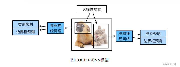
具体来说，R-CNN包括四个步骤：
1.对输入图像使用选择搜索来选取多个高质量的提议区域。
2.选择一个预训练的卷积神经网络，并将其在输出层之前截断。将每个提议区域变形为网络需要的输入尺寸，并通过前向传播输出抽取的提议区域特征。
3.将每个提议区域的特征连同其标注的类别作为一个样本。训练多个支持向量机对目标进行分类。
4.将每个提议区域的特征连同其标注的边界框作为一个样本，训练线性回归模型来预测真实边界框。

Fast R-CNN

1.相较于R-CNN模型，Fast R-CNN用来提取特征的卷积神经网络的输入是整个图像，而不是提议区域。
2.选择性搜索会生成若干个提议区域。引入了兴趣区域池化层：将卷积神经网络的输出和提议区域作为输入，输出连接后的各个提议区域抽取的特征。
3.通过全连接层将输出形状变换为n x d。
4.预测各个提议区的类别和边界框。
需要注意的是兴趣区域汇聚层将不同shape的输入汇聚成相同shape的输出。

# 例，其中spatial_scale=0.1,代表长宽的缩放。
torchvision.ops.roi_pool(X, rois, output_size=(2, 2), spatial_scale=0.1)
1
2

Faster R-CNN

为了较为精确地检测目标结果，Fast R-CNN模型需要在选择性搜索中生成大量地提议区域。Faster R-CNN提出将选择搜索替换成区域提议网络，从而减少提议区域地生成数量，并保证了精度。
区域提议网络的计算步骤为：
1.使用填充为1的3*3的卷积层变换卷积神经网络的输出。
2.以特征图的每个像素为中心，生成多个不同大小和宽高比的锚框。
3.使用锚框中心单元长度单元为c的特征，分别预测该锚框的二元类别和边界框。
4.使用非极大抑制，从预测类别为目标的预测边界框中移除相似的结果。最终输出即为所需的提议区域。

一阶段

单阶段模型没有中间的区域检出过程，直接从图片获得预测结果。

YOLO

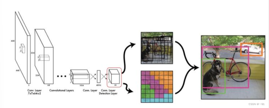
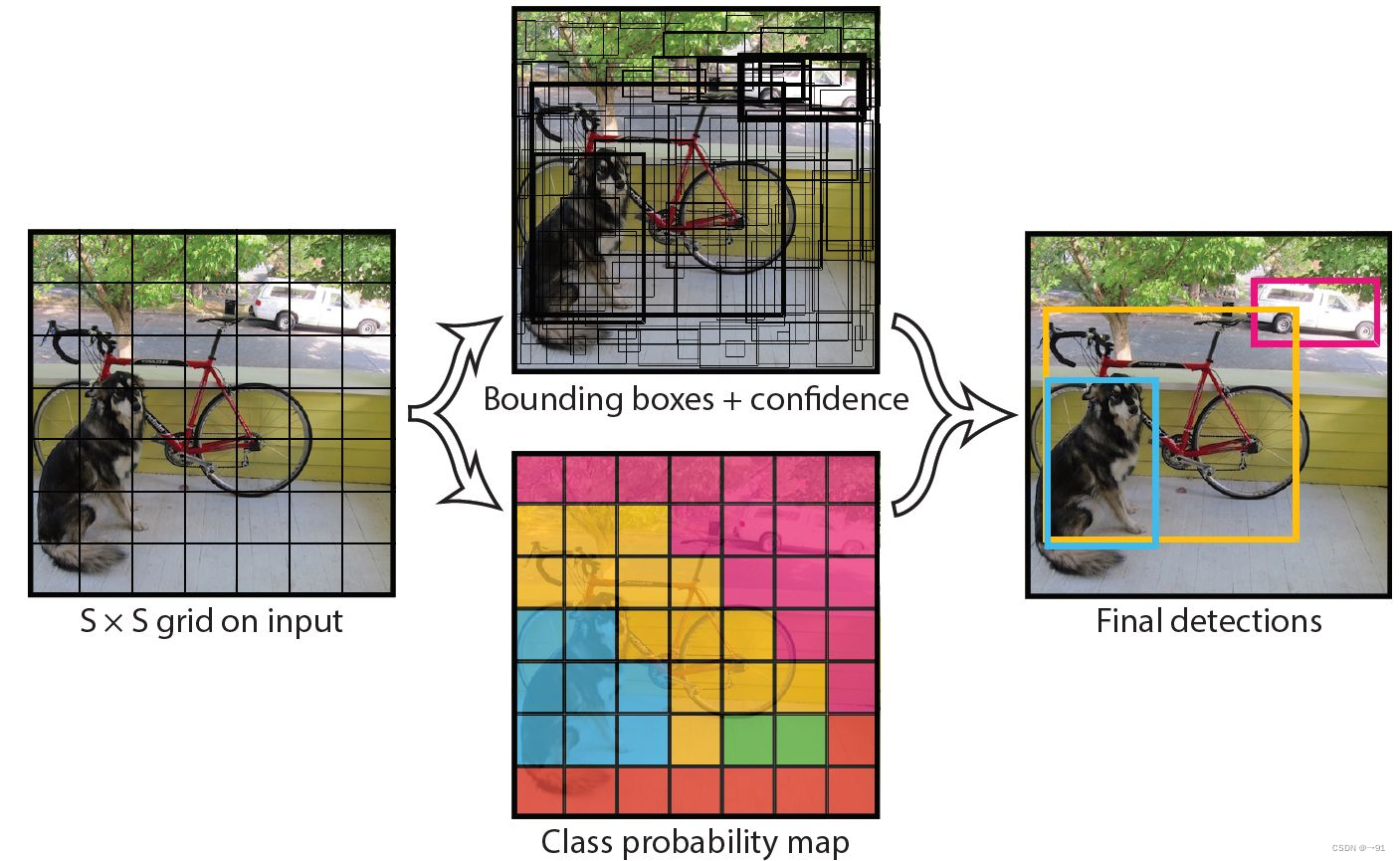
YOLO将检测任务表述为一个统一的、端到端的回归问题，即只处理图片一次同时得到位置和分类。
1.将图片输入CNN网络，将输入分割成S*S的网格。
2.每个单元格负责检测中心落在该格子内的目标。
3.每个单元格会预测B个边界框以及边界框的置信度。

SSD

1.基本网络用于从输入图像中提取特征。注：可以设计基础网络，使它输出的高和宽较大，可以用来检测尺寸较小的目标。
2.每个多尺度特征块将上一层提供的特征图的高和宽缩小（如减半），使特征图中每个单元在输入图像上有更广的感受野。
3.顶部的多尺度特征图较⼩，但具有较⼤的感受野，它们适合检测较少但较⼤的物体。
4.简⽽⾔之，通过多尺度特征块，单发多框检测⽣成不同⼤⼩的锚框，并通过预测边界框的类别和偏移量来检测⼤⼩不同的⽬标，因此这是⼀个多尺度⽬标检测模型。

三、项目实战

一、目标检测入门VOC2012

---