四、大数据实践——模型预测及分析

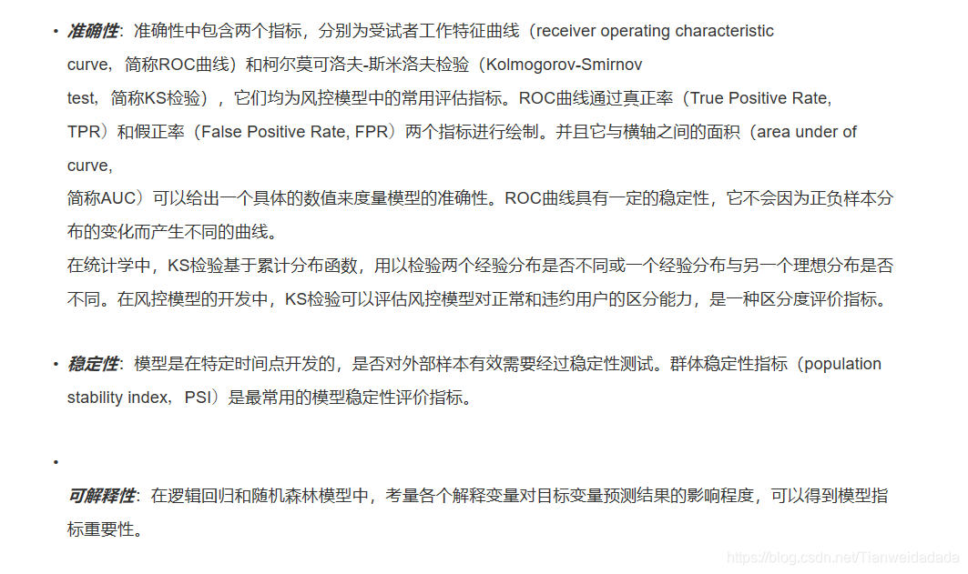
一、风险评估模型的效果评价方法

 

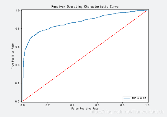
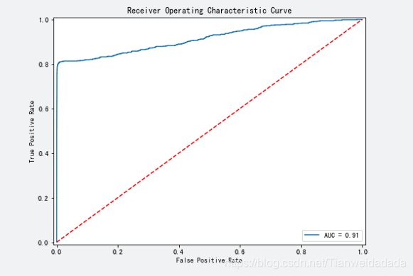
二、利用AUC评估逻辑回归模型的准确性

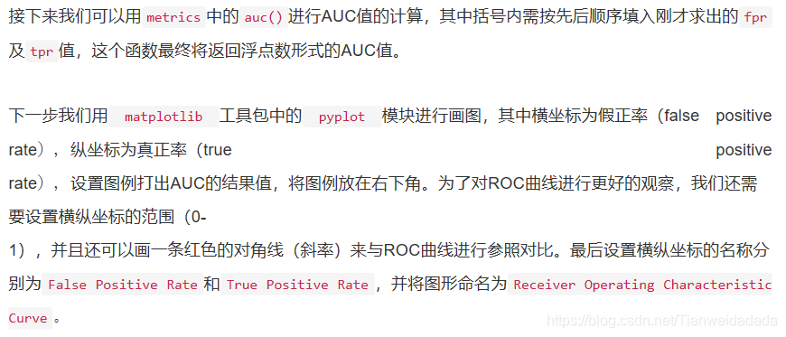
#用metrics.roc_curve()求出 fpr, tpr, threshold
fpr, tpr, threshold = metrics.roc_curve(y_test,y_predict_best)
 
#用metrics.auc求出roc_auc的值
roc_auc = metrics.auc(fpr,tpr)
 
#将图片大小设为8:6
fig,ax = plt.subplots(figsize=(8,6))
 
#将plt.plot里的内容填写完整
plt.plot(fpr, tpr, label = 'AUC = %0.2f' % roc_auc)
 
#将图例显示在右下方
plt.legend(loc = 'lower right') 
 
#画出一条红色对角虚线
plt.plot([0, 1], [0, 1],'r--') 
 
#设置横纵坐标轴范围
plt.xlim([-0.01, 1.01]) 
plt.ylim([-0.01, 1.01])
 
#设置横纵名称以及图形名称
plt.ylabel('True Positive Rate')
plt.xlabel('False Positive Rate')
plt.title('Receiver Operating Characteristic Curve')
plt.show()
 

三、利用AUC评估随机森林模型的准确性

#用metrics.roc_curve()求出 fpr, tpr, threshold
fpr, tpr, threshold = metrics.roc_curve(y_test,y_predict_best)
 
#用metrics.auc求出roc_auc的值
roc_auc = metrics.auc(fpr,tpr)
 
#将图片大小设为8:6
fig,ax = plt.subplots(figsize=(8,6))
 
#将plt.plot里的内容填写完整
plt.plot(fpr, tpr, label = 'AUC = %0.2f' % roc_auc)
 
#将图例显示在右下方
plt.legend(loc = 'lower right') 
 
#画出一条红色对角虚线
plt.plot([0, 1], [0, 1],'r--') 
 
#设置横纵坐标轴范围
plt.xlim([-0.01, 1.01]) 
plt.ylim([-0.01, 1.01])
 
#设置横纵名称以及图形名称
plt.ylabel('True Positive Rate')
plt.xlabel('False Positive Rate')
plt.title('Receiver Operating Characteristic Curve')
plt.show()
 

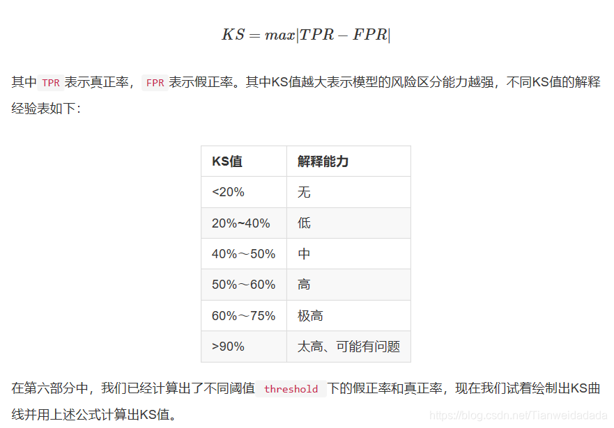
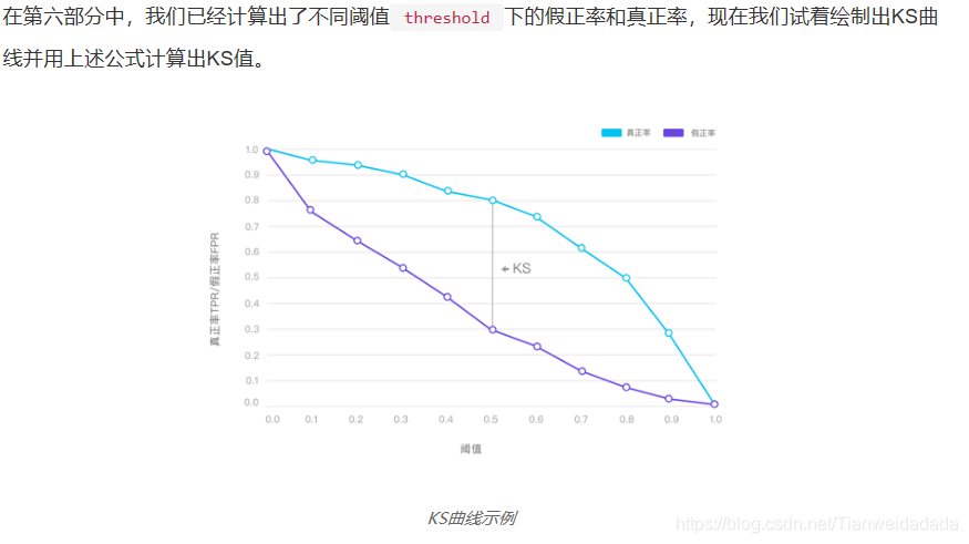
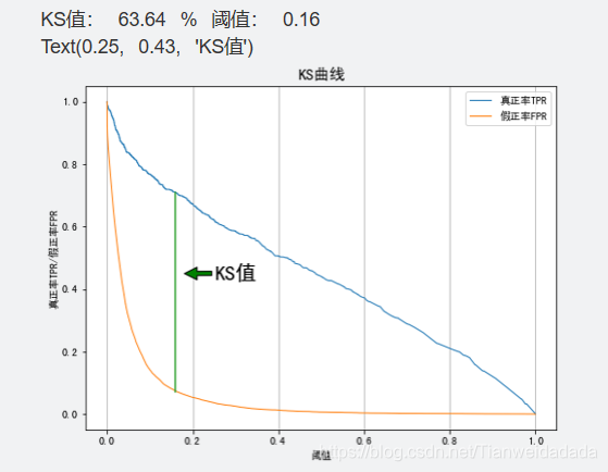
四、利用KS值评估逻辑回归模型的准确性

#用metric.roc_curve()求出 fpr, tpr, threshold
fpr, tpr, threshold = metrics.roc_curve(y_test, y_predict_best)
#print(threshold)
#求出KS值和相应的阈值
ks = max(abs(tpr-fpr))
thre = threshold[abs(tpr-fpr).argmax()]
 
ks = round(ks*100, 2)
thre = round(thre, 2)
print('KS值：', ks,  '%', '阈值：', thre)
 
#将图片大小设为8:6
fig = plt.figure(figsize=(8,6))
#将plt.plot里的内容填写完整
 
plt.plot(threshold[::-1], tpr[::-1], lw=1, alpha=1,label='真正率TPR')
plt.plot(threshold[::-1], fpr[::-1], lw=1, alpha=1,label='假正率FPR')
 
 
#画出KS值的直线
ks_tpr = tpr[abs(tpr-fpr).argmax()]
ks_fpr = fpr[abs(tpr-fpr).argmax()]
x1 = [thre, thre]
x2 = [ks_fpr, ks_tpr]
plt.plot(x1, x2)
 
#设置横纵名称以及图例
plt.xlabel('阈值')
plt.ylabel('真正率TPR/假正率FPR')
plt.title('KS曲线', fontsize=15)
plt.legend(loc="upper right")
plt.grid(axis='x')
 
# 在图上标注ks值
plt.annotate('KS值', xy=(0.18, 0.45), xytext=(0.25, 0.43),
             fontsize=20,arrowprops=dict(facecolor='green', shrink=0.01))

 五、利用KS值评估随机森林模型准确性（code同上）

六、利用PSI评估逻辑回归模型稳定性

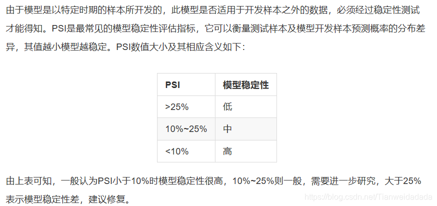
## 训练集预测概率
y_train_probs = lr.predict_proba(x_train)[:,1]
## 测试集预测概率
y_test_probs = lr.predict_proba(x_test)[:,1]
 
def psi(y_train_probs, y_test_probs):
    ## 设定每组的分点
    bins = np.arange(0, 1.1, 0.1)
    
    ## 将训练集预测概率分组
    y_train_probs_cut = pd.cut(y_train_probs, bins=bins, labels=False)
    ## 计算预期占比
    expect_prop = (pd.Series(y_train_probs_cut).value_counts()/len(y_train_probs)).sort_index()
    
    ## 将测试集预测概率分组
    y_test_probs_cut = pd.cut(y_test_probs, bins=bins, labels=False)
    ## 计算实际占比
    actual_prop = (pd.Series(y_test_probs_cut).value_counts()/len(y_test_probs)).sort_index()
    
    ## 计算PSI
    psi = ((actual_prop-expect_prop)*np.log(actual_prop/expect_prop)).sum
    
    return psi, expect_prop, actual_prop
 
## 运行函数得到psi、预期占比和实际占比
psi, expect_prop, actual_prop = psi(y_train_probs,y_test_probs)
print('psi=',psi)
 
## 创建(12, 8)的绘图框
fig = plt.figure(figsize=(12, 8))
 
## 设置中文字体
plt.rcParams['font.sans-serif'] = ['SimHei'] 
plt.rcParams['axes.unicode_minus'] = False
 
## 绘制条形图
plt.bar(expect_prop.index + 0.2, expect_prop, width=0.4, label='预期占比')
plt.bar(actual_prop.index - 0.2, actual_prop, width=0.4, label='实际占比')
plt.legend()
 
## 设置轴标签
plt.xlabel('概率分组', fontsize=12)
plt.ylabel('样本占比', fontsize=12)
 
## 设置轴刻度
plt.xticks([0, 1, 2, 3, 4, 5, 6, 7, 8, 9],
           ['0-0.1', '0.1-0.2', '0.2-0.3', '0.3-0.4', '0.4-0.5', '0.5-0.6', '0.6-0.7', '0.7-0.8', '0.8-0.9', '0.9-1'])
 
## 设置图标题
plt.title('预期占比与实际占比对比条形图', fontsize=15)
 
## 在图上添加文字
for index, item1, item2 in zip(range(10), expect_prop.values, actual_prop.values): 
    plt.text(index+0.2, item1 + 0.01, '%.3f' % item1, ha="center", va= "bottom",fontsize=10)
    plt.text(index-0.2, item2 + 0.01, '%.3f' % item2, ha="center", va= "bottom",fontsize=10)
 
 

七、计算逻辑回归指标重要性

 

 

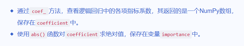
from sklearn.linear_model import LogisticRegression
lr_clf = LogisticRegression(penalty='l1',C = 0.6, random_state=55)
lr_clf.fit(x_train, y_train)
 
# 查看逻辑回归各项指标系数
coefficient = lr_clf.coef_
 
# 取出指标系数，并对其求绝对值
importance = abs(coefficient)
 
# 通过图形的方式直观展现前八名的重要指标
index=data.drop('Default', axis=1).columns
feature_importance = pd.DataFrame(importance.T, index=index).sort_values(by=0, ascending=True)
 
# # 查看指标重要度
print(feature_importance)
 
# 水平条形图绘制
feature_importance.tail(8).plot(kind='barh', title='Feature Importances', figsize=(8, 6), legend=False)
plt.show()

 八、计算随机森林的指标重要性

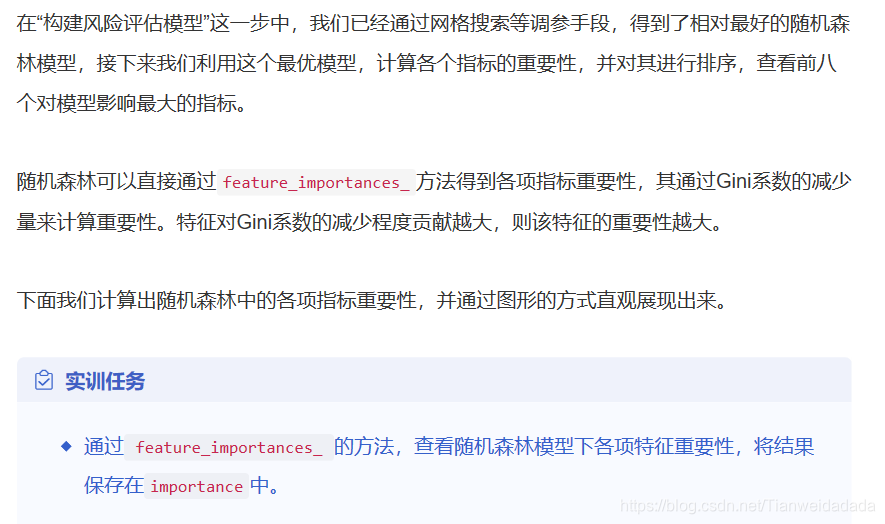
from sklearn.ensemble import RandomForestClassifier
rf = RandomForestClassifier(n_estimators = 150, criterion = 'entropy', max_depth = 5, min_samples_split = 2, random_state=12)
rf.fit(x_train, y_train)
 
# 查看随机森林各项指标系数
importance = rf.feature_importances_
 
# 通过图形的方式直观展现前八名的重要指标
index=data.drop('Default', axis=1).columns
feature_importance = pd.DataFrame(importance.T, index=index).sort_values(by=0, ascending=True)
 
# # 查看指标重要度
print(feature_importance)
 
# 水平条形图绘制
feature_importance.tail(8).plot(kind='barh', title='Feature Importances', figsize=(8, 6), legend=False)
plt.show()