【获奖复盘】2022年全国大学生数据分析大赛二等奖B题——Bert预训练模型与机器学习的餐饮情感二分类_情感分析二分类题目

这个比赛偶然在saike上看到的，不是很难比较水，由于是单人参赛，秉持着巩固锻炼一下自己的数据挖掘和机器学习水平的想法就报名了。由于赛题确实没什么含金量，7天的比赛3天我就把论文和代码写完了。不过也得益于我以前存过情感分析的深度学习bert模型代码，所以最后的训练效果非常好。最后离一等奖差了五名，有点遗憾但是也捞了个二等奖。给大家参考一下思路和代码吧

题目选择——题目 B：餐饮服务评价情感倾向分析

餐饮行业被誉为“永不落幕的黄金行业”，一方面是其“民以食为天”的刚需特性，另一方面是较低的创业门槛，使得行业竞争激烈。中国餐饮市场经过迅速发展，产业链逐步完善，餐饮外卖市场逐步成熟，在网络和疫情的影响下，年轻人的线上消费倾向进一步养成，很大程度上也助推了餐饮行业的线上发展。对餐饮企业来说，结合线上线下精细化运营，把握好用户评价，才能在竞争中脱颖而出。本题采集了不同餐饮企业的餐品评论数据，请根据提供的数据进行数据的清洗、分析与挖掘，并回答下列问题。

1. 对数据中的评价内容进行分析，制作词云图，分别给出积极情绪、消极情绪评价次数最多的 10 个词。
2. 分析数据中用户评价的积极情绪、消极情绪与评价时间是否存在关系，请说明理由。
3. 积极情绪最多的是哪个商家，并总结这个商家的优点有哪些。
4. 消极情绪最多的是哪个商家，并提出相关改进策略，提高顾客的积极情绪。
5. 建立餐饮服务评论的情感倾向模型，并对模型的性能和误差进行评估。基于模型对附件中的测试数据 test.xlsx 进行评测，将评测结果补充到第一列中，并将此文件一起上传到竞赛平台。

题目分析

题意非常简单，前四个都是初学者都会的难度，制作词云图，分析关系，一些语言处理的操作。唯一有坑的一点是第二问中存在关系的判断，需要对时间属性进行特征工程。
而第五问，我用机器学习方法和深度学习bert模型+lstm对数据集进行训练对效果进行了对比，最后深度学习的准确率高达96.1%，且没有过拟合的现象。
我这里分享出我的摘要：

在如今互联网企业高速发展与疫情爆发的影响下，点外卖逐渐成为了当代年轻人生活中不可或缺的一环。中国餐饮市场经过迅速发展，产业链逐步完善，餐饮外卖市场也走向了“内卷”。对餐饮企业来说，结合线上与线下精细化运营，把握好用户评价，才能在竞争中脱颖而出。
首先，我对数据集进行数据预处理与特征工程操作。利用正则表达式去除评价文本中的特殊符号，对评论时间属性进行了特征工程，并对各项属性进行了可视化分析。
对于问题一，将处理后的评价文本利用 python 的jieba 库进行分词并去除停用词。将分词后的文本生成词典并统计词频。通过统计的词频输出积极与消极情绪评价次数最多的十个词，并制作了相应的词云图。
对于问题二，将先前特征工程后的评价时间属性抽出两个连续变量：一年中的第几天和一天中的第几秒。使用 Point-biserial 系数计算二分类变量与这两个连续变量之间的相关性，得出结论消极情绪与积极情绪在评价时间上不存在明显关系。
对于问题三，通过 pandas 的查找函数我发现编号1041 商家拥有54 条最多的好评。根据该商家的评论文本进行分词分析后发现该商家的优点为：菜品味道好，价格实惠，包装精致，服务到位，送餐速度快。
对于问题四，通过 pandas 的查找函数我发现编号971 商家店家50 条评论中有 44 条消极差评为所有商家中最多。根据差评中的痛点分析后，我提出了针对配送速度，菜品口味，商家服务这三个问题的 7 种改进策略。
对于问题五，首先将分词处理后的文本进行词向量的形式转换，以7 比3划分训练集与测试集，再选用了随机森林，支持向量机，梯度提升树三种典型机器学习分类算法进行模型构建。通过对比各项评价指标，支持向量机以89%的准确率，召回率与 F1-score 略优于其他模型。最后，我选用了深度学习中的Bert+Bi-LSTM 模型，对其针对问题进行改良，运用哈工大中文Bert 预训练权重作为基础，最后的测试集准确率高达 96.1%，相较于机器学习提高了接近7%。并基于训练后的模型对测试数据进行了评测。
通过对用户评价数据集的分析，我们可以从中挖掘出用户的潜在喜好与属性。先通过数据挖掘和数据处理方法对数据集进行深入处理与理解，再利用机器学习和深度学习的方法对用户的积极与消极情绪进行二元情感预测分类。从而让商家能够更好的运营与分析线上平台的用户评价，更好的服务并满足用户需求，提升品牌价值。
关键词：特征工程 相关性分析 词向量 深度学习 Bert Bi-LSTM机器学习

部分代码

代码语言全部为Python且用jupyter notebook编写，下面是论文中部分操作的代码

1.引入需要的库文件

%matplotlib inline
import numpy as np 
import pandas as pd
import matplotlib.pyplot as plt
import seaborn as sns
import os
import re

from sklearn.model_selection import train_test_split 
import jieba
import nltk
from sklearn.ensemble import RandomForestClassifier, GradientBoostingClassifier
import time
import scipy
from nltk.classify import SklearnClassifier
from sklearn.svm import LinearSVC
from sklearn.naive_bayes import MultinomialNB
from sklearn.ensemble import GradientBoostingClassifier
from sklearn.linear_model import Perceptron

from wordcloud import WordCloud,STOPWORDS
import warnings
warnings.filterwarnings('ignore')

# 中文乱码的处理
plt.rcParams['font.sans-serif'] =['Microsoft YaHei']
plt.rcParams['axes.unicode_minus'] = False
1
2
3
4
5
6
7
8
9
10
11
12
13
14
15
16
17
18
19
20
21
22
23
24
25
26
27

2.读取数据

data = pd.read_excel("./data/data.xlsx")
data.head()

test = pd.read_excel("./data/test.xlsx")
test.head()

1
2
3
4
5
6

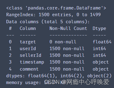
字段 说明:
target: 评价标签，0为积极情绪，1为消极情绪
userId: 用户id，对应每个用户
sellerId: 商家id，对应每个商家
timestamp: 评价的时间
comment: 评价的内容

test.info()
# 没有空缺值
data.isnull().sum().max()
1
2
3

3.文本预处理

可以看到data和test的comment里的文本前后都有一些和文本无关的字符比如(text:, \n, 特殊符号)

data['comment'] = data['comment'].str.strip("text：")
test['comment'] = test['comment'].str.strip("text：")
1
2

利用正则表达式去除文本中的标点符号

data['comment'] = data['comment'].apply(
 lambda x: re.sub('[^\u4E00-\u9FD5,.?!，。！？、；;:：0-9]+', '', x)
)

test['comment'] = test['comment'].apply(
 lambda x: re.sub('[^\u4E00-\u9FD5,.?!，。！？、；;:：0-9]+', '', x)
)
1
2
3
4
5
6
7

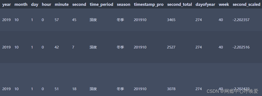
4.特征工程

timestamp属性处理

# 年份
data['year']=data['timestamp'].apply(lambda x: x.year)
 
# 月份
data['month']=data['timestamp'].apply(lambda x: x.month)
 
# 日
data['day']=data['timestamp'].apply(lambda x: x.day)
 
# 小时
data['hour']=data['timestamp'].apply(lambda x: x.hour)
 
# 分钟
data['minute']=data['timestamp'].apply(lambda x: x.minute)
 
# 秒数
data['second']=data['timestamp'].apply(lambda x: x.second)

data['second_total_day'] = data['timestamp'].apply(lambda x: x.second + x.minute*60 + x.hour*60*60)
period_dict ={
    23: '深夜', 0: '深夜', 1: '深夜',
    2: '凌晨', 3: '凌晨', 4: '凌晨',
    5: '早晨', 6: '早晨', 7: '早晨',
    8: '上午', 9: '上午', 10: '上午', 11: '上午',
    12: '中午', 13: '中午',
    14: '下午', 15: '下午', 16: '下午', 17: '下午',
    18: '傍晚',
    19: '晚上', 20: '晚上', 21: '晚上', 22: '晚上',
}
data['time_period']=data['hour'].map(period_dict)
season_dict = {
    1: '春季', 2: '春季', 3: '春季',
    4: '夏季', 5: '夏季', 6: '夏季',
    7: '秋季', 8: '秋季', 9: '秋季',
    10: '冬季', 11: '冬季', 12: '冬季',
}
data['season']=data['month'].map(season_dict)

data['timestamp_pro']= data['timestamp'].apply(lambda x: str(x.year)+str(x.month))
# 一年中的第几天
data['dayofyear']=data['timestamp'].apply(lambda x: x.dayofyear)

# 一年中的第几周
data['week']=data['timestamp'].apply(lambda x: x.week)
1
2
3
4
5
6
7
8
9
10
11
12
13
14
15
16
17
18
19
20
21
22
23
24
25
26
27
28
29
30
31
32
33
34
35
36
37
38
39
40
41
42
43
44

5.可视化操作

评论情感分布

plt.style.use('fivethirtyeight')
val_count = data['target'].value_counts()

plt.figure(figsize=(8,4))
sns.countplot(data=data, x='target')
plt.title("Sentiment Data Distribution")
1
2
3
4
5
6

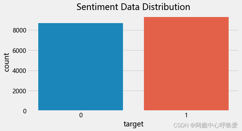
分析：对评论在积极与消极情绪属性上进行绘图。其中积极情绪(0)评论有8672条，消极情绪(1)评论有 9281 条。比例上接近 1 比 1，说明给出的数据集类别相对均衡，不需要对数据集类别上做额外工作。

商家评论分布

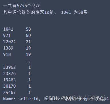
Seller = data['sellerId'].value_counts()
print("一共有{}个商家".format(len(Seller.index)))
print("其中评论最多的商家id是：",Seller.index[0],"为58条")
Seller
1
2
3
4

plt.pie(Seller.values[:10], labels=SellerIndex[:10], autopct='%1.1f%%', counterclock=False, startangle=90, explode=[0.1,0,0,0,0,0,0,0,0,0])
plt.title("前十家评论最多的店铺-饼图")
plt.tight_layout()
plt.show()
1
2
3
4

分析：通过 pandas 的 value_counts 函数，对数据集进行初步分析。在数据集中一共有 5745 个商家，大部分的店家的评论数较少。其中评论最多的商家是1041共有 58 条评论。商家的评论越多说明商家越火爆，话题度也越高，分析其情感分布可以帮助用户更好的选择优质店铺。

评论时间分布

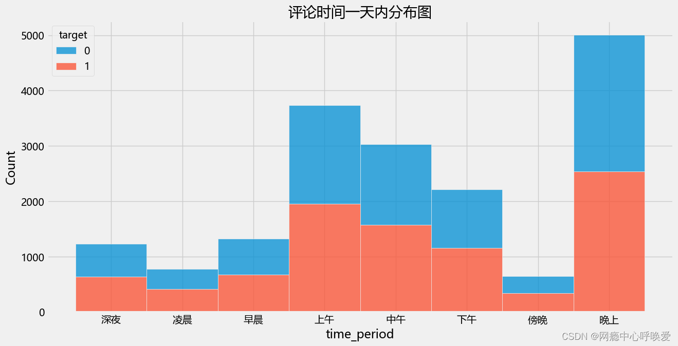
plt.figure(figsize=(14,7))
sns.histplot(data=data, x='time_period', hue='target', multiple='stack')
plt.title("评论时间一天内分布图")
plt.show()
1
2
3
4

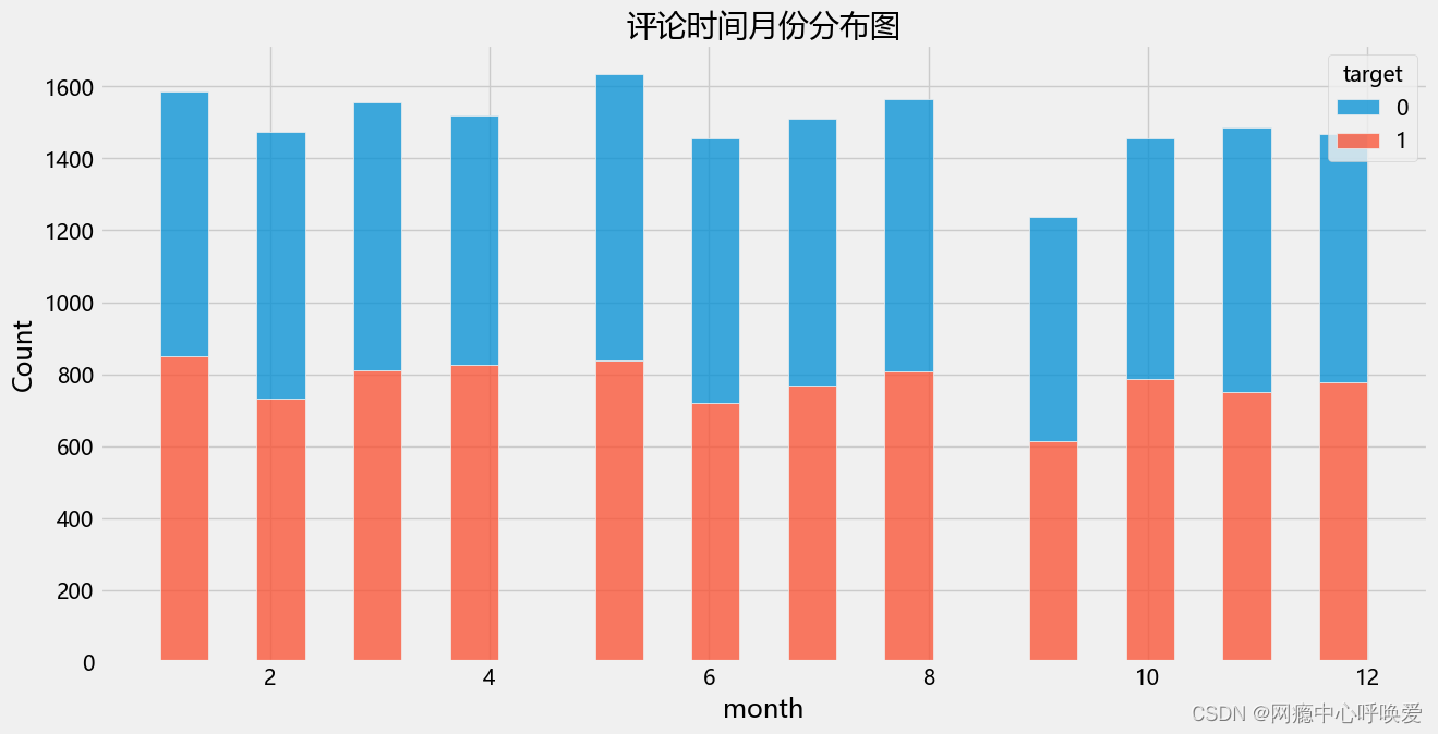
plt.figure(figsize=(14,7))
sns.histplot(data=data, x='month', hue='target', multiple='stack')
plt.title("评论时间月份分布图")
plt.show()
1
2
3
4

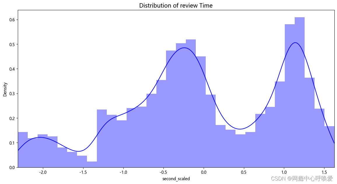
fig, ax = plt.subplots(1, 1, figsize=(14, 7))

time_val = data['second_scaled']

sns.distplot(time_val, ax=ax, color='b')
ax.set_title('Distribution of review Time', fontsize=14)
ax.set_xlim([min(time_val), max(time_val)])

plt.show()
1
2
3
4
5
6
7
8
9

分析：从时间属性上来看，数据集的评论时间从 2019 年10 月1 日0 点到2020年 9 月 27 日的 23:59。整个时间戳在一天的时间段上是不间断的从0 点到23点，而在时间跨度上为 364 天。在不同的季节中，评论数量略有波动，春季和夏季略多一些；其中积极与消极情绪比例接近 1 比 1。在不同的时间段上，评论数量差异较大，评论主要集中于 8-13 点的上午中午时间段以及19- 22 点的晚上时间段；其中积极与消极的比例接近 1 比 1。这些结果印证了我在特征工程阶段的时间分布图表。

6.时间相关性

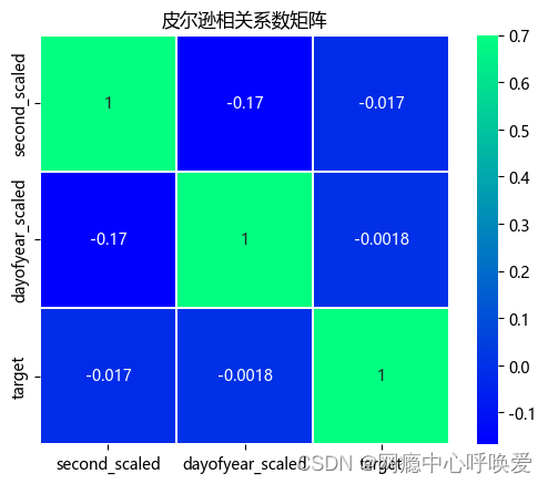
由于在第二部分特征工程阶段，我们发现了在时间上数据集跨越了364 天即一年的连续时间段，以及一天内的时间也从 0 点持续到24 点，都是连续的。所以我将重点关注探讨 dayofyear(一年中的第几天)，以及从second_total_day（一
天中的第几秒）这两个评价时间属性和积极与消极情绪分类属性之间的相关性分析。
由于一边是二分类属性，一边是连续数值，常用的皮尔逊相关系数的并不适用这种条件，所以我改用了点二系列相关系数(Point-biserial correlation)。Point-biserial 相关适用于分析二分类变量和连续变量之间的相关性是Pearson相关的一种特殊形式，与 Pearson 相关的数据假设一致。通过 Python 的 scipy 库的 stats 模块调用 pointbiserialr 函数可以计算出属性之间两两的相关系数。根据下图 18 可以得出，target 属性与dayofyear_scaled和second_total_day_scaled 属性之间的相关系数的绝对值小于0.1 说明几乎没有相关性。所以我得出结论：用户评价的积极情绪、消极情绪与评价时间不存在明显关系。

1.皮尔逊相关系数

from sklearn.preprocessing import StandardScaler

ss = StandardScaler() 
data['second_scaled'] = ss.fit_transform(data['second_total_day'].values.reshape(-1,1))

data['dayofyear_scaled'] = ss.fit_transform(data['dayofyear'].values.reshape(-1,1))
data_time = data[['second_scaled','dayofyear_scaled','target']]
plt.title('皮尔逊相关系数矩阵')
sns.heatmap(data_time.corr(),linewidths=0.25,vmax=0.7,square=True,cmap="winter",
            linecolor='w',annot=True);
1
2
3
4
5
6
7
8
9
10

2. 点二系列相关系数(Point-biserial correlation)

scipy.stats.pointbiserialr(data['target'].values, data['second_scaled'].values)
scipy.stats.pointbiserialr(data['target'].values, data['dayofyear_scaled'].values)
1
2

7.词云绘制

分词&&去除停用词

#获取停用词列表
def getStopWords(file_name):
    stop_words = []                                       #定义停用词表

    with open(file_name, 'r', encoding='UTF-8') as fp:
        stop_words = fp.read().split('\n')                #读取所有停用词，并存放到列表中
        
    return stop_words                                    #返回停用词列表

#去处停用词，并返回评论切分后的评论列表，每个元素均为一个词语列表
def removeStopWords(X, stop_words):
    all_words = []                                        #定义存放评论的列表，评论均以词典列表形式存在
    
    for sentence in X:                                    #遍历评论列表
        words = []                                        #存放每个评论词语的列表
        
        for word in jieba.lcut(sentence):                 #遍历评论分词后的列表
            
            if word not in stop_words:                    #该词语未在停用词表中
                words.append(word)                         #追加到words中，实现去停用词
                
        all_words.append(words)                            #总评论列表追加该评论分词列表
    
    return all_words                                      #返回结果


stopwords_path = './data/hit_stopwords.txt'
stopwords_List = getStopWords(stopwords_path)
print("一共有",len(stopwords_List),"条停用词")
stopwords_List
1
2
3
4
5
6
7
8
9
10
11
12
13
14
15
16
17
18
19
20
21
22
23
24
25
26
27
28
29
30

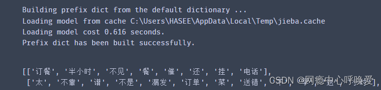
comment_cut = removeStopWords(comment.values, stopwords_List)
comment_cut[:5]
1
2

生成词典与词频统计

#生成词典，存放评论中所有出现过的词语，待统计词频
def getDictionary(X):
    dictionary = []                                        #定义词典，存放所有出现过的词语
    
    for sentence in X:
        for word in sentence:
            if word not in dictionary:                    #遍历所有评论的词语，若未在词典中存在
                dictionary.append(word)                    #添加
    
    return dictionary                                     #返回结果
comment_dic_pos = getDictionary(comment_cut_pos)
comment_dic_neg = getDictionary(comment_cut_neg)
comment_dic = getDictionary(comment_cut)
1
2
3
4
5
6
7
8
9
10
11
12
13

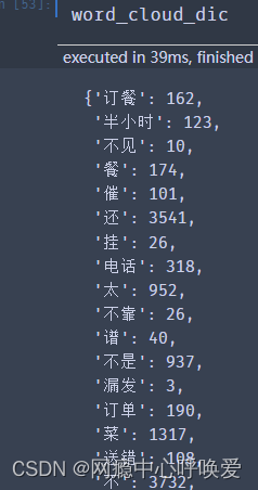
# 统计每个词出现的次数
word_cloud_dic = {}
for sentence in comment_cut:
    for w in sentence:
        if w in word_cloud_dic.keys():
            word_cloud_dic[w] = word_cloud_dic[w]+1
        else:
            word_cloud_dic[w] = 1
1
2
3
4
5
6
7
8

# 统计每个词出现的次数
word_cloud_dict_pos = {}
for sentence in comment_cut_pos:
    for w in sentence:
        if w in word_cloud_dict_pos.keys():
            word_cloud_dict_pos[w] = word_cloud_dict_pos[w]+1
        else:
            word_cloud_dict_pos[w] = 1
      
word_cloud_dict_neg = {}
for sentence in comment_cut_neg:
    for w in sentence:
        if w in word_cloud_dict_neg.keys():
            word_cloud_dict_neg[w] = word_cloud_dict_neg[w]+1
        else:
            word_cloud_dict_neg[w] = 1
1
2
3
4
5
6
7
8
9
10
11
12
13
14
15
16

绘制词云图

word_cloud_data = sorted(word_cloud_dic.items(),key=lambda x:x[1],reverse=True)
word_cloud_data[:10]
1
2

# 绘制词云
my_cloud = WordCloud(
    background_color='white',  # 设置背景颜色  默认是black
    width=800, height=500,
    max_words=150,            # 词云显示的最大词语数量
    font_path='simhei.ttf',   # 设置字体  显示中文
    max_font_size=99,         # 设置字体最大值
    min_font_size=16,         # 设置子图最小值
    random_state=50           # 设置随机生成状态，即多少种配色方案
).generate_from_frequencies(word_cloud_dic)
 
# 显示生成的词云图片
plt.imshow(my_cloud, interpolation='bilinear')
# 显示设置词云图中无坐标轴
plt.axis('off')
plt.show()
1
2
3
4
5
6
7
8
9
10
11
12
13
14
15
16

8.机器学习

转换为词向量

comment = data['comment']
comment.values
1
2

#通过词袋模型将每条评论均转换为对应的向量，返回
def word_2_vec(X, dictionary):
    n = len(dictionary)                                   #词典长度
    
    word_vecs = []                                        #存放所有向量的列表
    
    for sentence in X:                                    #遍历评论列表
        word_vec = np.zeros(n)                            #生成 (1,n)维的 0向量
        for word in sentence:                             #遍历评论中的所有词语
            if word in dictionary:                        #若该词语在字典中
                loc = dictionary.index(word)              #找到在词典中的位置
                word_vec[loc] += 1                        #为向量的此位置累加1
            
        word_vecs.append(word_vec)                      #评论列表累加向量
        
    return np.array(word_vecs)                                     #返回结果
1
2
3
4
5
6
7
8
9
10
11
12
13
14
15
16

划分数据集

from sklearn import metrics
from sklearn.metrics import precision_score, recall_score, f1_score, roc_auc_score, accuracy_score, classification_report
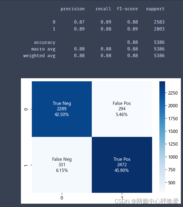
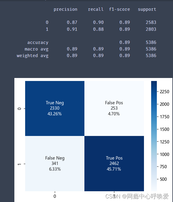
# 绘制混淆矩阵
def model_evaluation(classifier,x_test,y_test):  
    
    cm = metrics.confusion_matrix(y_test,classifier.predict(x_test))
    names = ['True Neg','False Pos','False Neg','True Pos']
    counts = [value for value in cm.flatten()]
    percentages = ['{0:.2%}'.format(value) for value in cm.flatten()/np.sum(cm)]
    labels = [f'{v1}\n{v2}\n{v3}' for v1, v2, v3 in zip(names,counts,percentages)]
    labels = np.asarray(labels).reshape(2,2)
    sns.heatmap(cm,annot = labels,cmap = 'Blues',fmt ='')
    
    print(classification_report(y_test,classifier.predict(x_test)))
1
2
3
4
5
6
7
8
9
10
11
12
13
14

# X = data['comment_cut']    #取出所有评论信息
y = data['target']           #取出所有标签信息

X = word_2_vec(comment_cut, comment_dic)    #将评论内容通过词袋模型转化为向量

X_train, X_test, y_train, y_test = train_test_split(X, y, test_size=0.30, shuffle=True, random_state=42)    #拆分数据集为训练集、测试集(7:3)
1
2
3
4
5
6

随机森林

forest = RandomForestClassifier(n_estimators=100)                     #构造随机森林，共存在100棵树
forest.fit(X_train, y_train)                                            #训练数据

res01 = forest.score(X_train, y_train)                    #评估训练集的准确度
res02 = forest.score(X_test, y_test)                      #评估测试集的准确度

print('The training: {}'.format(res01))
print('The test: {}'.format(res02))                       #输出结果
1
2
3
4
5
6
7
8

model_evaluation(forest, X_test, y_test)
1

朴素贝叶斯

native_bayes = MultinomialNB()
native_bayes.fit(X_train, y_train)                              #训练数据


res_train = native_bayes.score(X_train, y_train)                    #评估训练集的准确度
res_test = native_bayes.score(X_test, y_test)                      #评估测试集的准确度


print('The training: {}'.format(res_train))
print('The test: {}'.format(res_test))                       #输出结果
model_evaluation(native_bayes, X_test, y_test)
1
2
3
4
5
6
7
8
9
10
11

9.深度学习Bert模型

初步准备

由于我们的评价文本都是中文，所以我选择了哈工大中文bert 预训练模型作为本深度学习模型的基础。在 huggingface 官网下载 pytorch 版权重，并在conda环境中安装 Transformers 库，进行初步准备。

模型设置

pip install transformers

import pandas as pd
import numpy as np
import torch
import torch.nn as nn
import torch.nn.functional as F
from transformers import BertTokenizer,BertModel
from torch.utils.data import TensorDataset, DataLoader
from sklearn.model_selection import train_test_split
import re
1
2
3
4
5
6
7
8
9
10
11

np.random.seed(0)
torch.manual_seed(0)
USE_CUDA = torch.cuda.is_available()
if USE_CUDA:
    torch.cuda.manual_seed(0)
1
2
3
4
5

#剔除标点符号,\xa0 空格
def pretreatment(comments):
    result_comments=[]
    punctuation='。，？！：%&~（）、；“”&|,.?!:%&~();""'
    for comment in comments:
        comment= ''.join([c for c in comment if c not in punctuation])
        comment= ''.join(comment.split())   #\xa0
        result_comments.append(comment)
    
    return result_comments
1
2
3
4
5
6
7
8
9
10

模型定义

class bert_lstm(nn.Module):
    def __init__(self, bertpath, hidden_dim, output_size,n_layers,bidirectional=True, drop_prob=0.5):
        super(bert_lstm, self).__init__()
 
        self.output_size = output_size
        self.n_layers = n_layers
        self.hidden_dim = hidden_dim
        self.bidirectional = bidirectional
        
        #Bert ----------------重点，bert模型需要嵌入到自定义模型里面
        self.bert=BertModel.from_pretrained(bertpath)
        for param in self.bert.parameters():
            param.requires_grad = True
        
        # LSTM layers
        self.lstm = nn.LSTM(768, hidden_dim, n_layers, batch_first=True,bidirectional=bidirectional)
        
        # dropout layer
        self.dropout = nn.Dropout(drop_prob)
        
        # linear and sigmoid layers
        if bidirectional:
            self.fc = nn.Linear(hidden_dim*2, output_size)
        else:
            self.fc = nn.Linear(hidden_dim, output_size)
          
        #self.sig = nn.Sigmoid()
 
    def forward(self, x, hidden):
        batch_size = x.size(0)
        #生成bert字向量
        x=self.bert(x)[0]     #bert 字向量
        
        # lstm_out
        #x = x.float()
        lstm_out, (hidden_last,cn_last) = self.lstm(x, hidden)
        #print(lstm_out.shape)   #[32,100,768]
        #print(hidden_last.shape)   #[4, 32, 384]
        #print(cn_last.shape)    #[4, 32, 384]
        
        #修改 双向的需要单独处理
        if self.bidirectional:
            #正向最后一层，最后一个时刻
            hidden_last_L=hidden_last[-2]
            #print(hidden_last_L.shape)  #[32, 384]
            #反向最后一层，最后一个时刻
            hidden_last_R=hidden_last[-1]
            #print(hidden_last_R.shape)   #[32, 384]
            #进行拼接
            hidden_last_out=torch.cat([hidden_last_L,hidden_last_R],dim=-1)
            #print(hidden_last_out.shape,'hidden_last_out')   #[32, 768]
        else:
            hidden_last_out=hidden_last[-1]   #[32, 384]
            
            
        # dropout and fully-connected layer
        out = self.dropout(hidden_last_out)
        #print(out.shape)    #[32,768]
        out = self.fc(out)
        
        return out
    
    def init_hidden(self, batch_size):
        weight = next(self.parameters()).data
        
        number = 1
        if self.bidirectional:
            number = 2
        
        if (USE_CUDA):
            hidden = (weight.new(self.n_layers*number, batch_size, self.hidden_dim).zero_().float().cuda(),
                      weight.new(self.n_layers*number, batch_size, self.hidden_dim).zero_().float().cuda()
                     )
        else:
            hidden = (weight.new(self.n_layers*number, batch_size, self.hidden_dim).zero_().float(),
                      weight.new(self.n_layers*number, batch_size, self.hidden_dim).zero_().float()
                     )
        
        return hidden
1
2
3
4
5
6
7
8
9
10
11
12
13
14
15
16
17
18
19
20
21
22
23
24
25
26
27
28
29
30
31
32
33
34
35
36
37
38
39
40
41
42
43
44
45
46
47
48
49
50
51
52
53
54
55
56
57
58
59
60
61
62
63
64
65
66
67
68
69
70
71
72
73
74
75
76
77
78
79

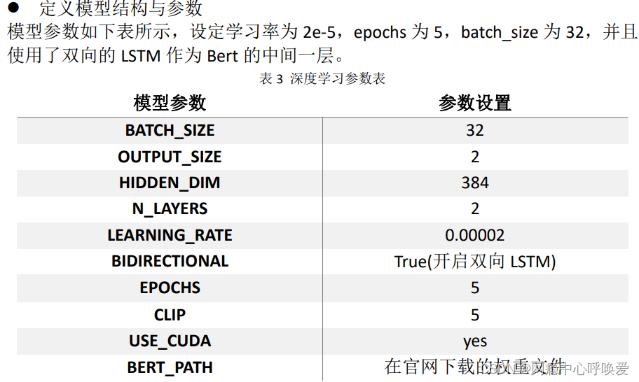
模型参数设置

class ModelConfig:
    batch_size = 32
    output_size = 2
    hidden_dim = 384   #768/2
    n_layers = 2
    lr = 0.00002 #0.00002
    bidirectional = True  #这里为True，为双向LSTM
    # training params
    epochs = 5
    # batch_size=50
    print_every = 10
    clip=5 # gradient clipping
    use_cuda = USE_CUDA
    bert_path = './drive/MyDrive/bert-base-chinese' #预训练bert路径
    save_path = './drive/MyDrive/bert_bilstm2.pth' #模型保存路径
1
2
3
4
5
6
7
8
9
10
11
12
13
14
15

模型训练设置

def train_model(config, data_train):
    net = bert_lstm(config.bert_path, 
                    config.hidden_dim, 
                    config.output_size,
                    config.n_layers, 
                    config.bidirectional)
    criterion = nn.CrossEntropyLoss()
    optimizer = torch.optim.Adam(net.parameters(), lr=config.lr)
    if(config.use_cuda):
        net.cuda()
    net.train()
    for e in range(config.epochs):
        # initialize hidden state
        h = net.init_hidden(config.batch_size)
        counter = 0
        # batch loop
        for inputs, labels in data_train:
            counter += 1
            
            if(config.use_cuda):
                inputs, labels = inputs.cuda(), labels.cuda()
            h = tuple([each.data for each in h])
            net.zero_grad()
            output= net(inputs, h)
            loss = criterion(output.squeeze(), labels.long())
            loss.backward()
            optimizer.step()
    
            # loss stats
            if counter % config.print_every == 0:
                net.eval()
                with torch.no_grad():
                    val_h = net.init_hidden(config.batch_size)
                    val_losses = []
                    for inputs, labels in valid_loader:
                        val_h = tuple([each.data for each in val_h])

                        if(config.use_cuda):
                            inputs, labels = inputs.cuda(), labels.cuda()

                        output = net(inputs, val_h)
                        val_loss = criterion(output.squeeze(), labels.long())

                        val_losses.append(val_loss.item())
                net.train()
                train_loss_list.append(loss.item())
                train_val_loss_list.append(np.mean(val_losses))
                print("Epoch: {}/{}, ".format(e+1, config.epochs),
                    "Step: {}, ".format(counter),
                    "Loss: {:.6f}, ".format(loss.item()),
                    "Val Loss: {:.6f}".format(np.mean(val_losses)))
    torch.save(net.state_dict(), config.save_path)
1
2
3
4
5
6
7
8
9
10
11
12
13
14
15
16
17
18
19
20
21
22
23
24
25
26
27
28
29
30
31
32
33
34
35
36
37
38
39
40
41
42
43
44
45
46
47
48
49
50
51
52

模型测试设置

def test_model(config, data_test):
    net = bert_lstm(config.bert_path, 
                config.hidden_dim, 
                config.output_size,
                config.n_layers, 
                config.bidirectional)
    net.load_state_dict(torch.load(config.save_path))
    net.cuda()
    criterion = nn.CrossEntropyLoss()
    test_losses = [] # track loss
    num_correct = 0
    
    # init hidden state
    h = net.init_hidden(config.batch_size)
    
    net.eval()
    # iterate over test data
    for inputs, labels in data_test:
        h = tuple([each.data for each in h])
        if(USE_CUDA):
            inputs, labels = inputs.cuda(), labels.cuda()
        output = net(inputs, h)
        test_loss = criterion(output.squeeze(), labels.long())
        test_losses.append(test_loss.item())
        
        output=torch.nn.Softmax(dim=1)(output)
        pred=torch.max(output, 1)[1]
        
        # compare predictions to true label
        # print(pred)
        correct_tensor = pred.eq(labels.long().view_as(pred))
        correct = np.squeeze(correct_tensor.numpy()) if not USE_CUDA else np.squeeze(correct_tensor.cpu().numpy())
        num_correct += np.sum(correct)
    print("Test loss: {:.3f}".format(np.mean(test_losses)))
    # accuracy over all test data
    test_acc = num_correct/len(data_test.dataset)
    print("Test accuracy: {:.3f}".format(test_acc))
1
2
3
4
5
6
7
8
9
10
11
12
13
14
15
16
17
18
19
20
21
22
23
24
25
26
27
28
29
30
31
32
33
34
35
36
37

模型预测设置

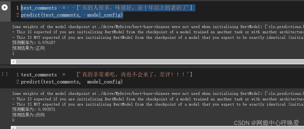
def predict(test_comment_list, config):
    net = bert_lstm(config.bert_path, 
                config.hidden_dim, 
                config.output_size,
                config.n_layers, 
                config.bidirectional)
    net.load_state_dict(torch.load(config.save_path))
    net.cuda()
    result_comments=pretreatment(test_comment_list)   #预处理去掉标点符号
    #转换为字id
    tokenizer = BertTokenizer.from_pretrained(config.bert_path)
    result_comments_id = tokenizer(result_comments,
                                    padding=True,
                                    truncation=True,
                                    max_length=120,
                                    return_tensors='pt')
    tokenizer_id = result_comments_id['input_ids']
    # print(tokenizer_id.shape)
    inputs = tokenizer_id
    batch_size = inputs.size(0)
    # batch_size = 32
    # initialize hidden state
    h = net.init_hidden(batch_size)
    

    if(USE_CUDA):
        inputs = inputs.cuda()

    net.eval()
    with torch.no_grad():
        # get the output from the model
        output= net(inputs, h)
        output=torch.nn.Softmax(dim=1)(output)
        pred=torch.max(output, 1)[1]
        # printing output value, before rounding
        print('预测概率为: {:.6f}'.format(torch.max(output, 1)[0].item()))
        if(pred.item()==1):
            print("预测结果为:负向")
            pred_res = 0
        else:
            print("预测结果为:正向")
            pred_res = 1
    return pred_res
1
2
3
4
5
6
7
8
9
10
11
12
13
14
15
16
17
18
19
20
21
22
23
24
25
26
27
28
29
30
31
32
33
34
35
36
37
38
39
40
41
42
43

开始训练

if __name__ == '__main__':
    model_config = ModelConfig()
    data=pd.read_excel('data.xlsx')
    data['comment'] = data['comment'].str.strip("text：")
    data['comment'] = data['comment'].apply(lambda x: re.sub('[^\u4E00-\u9FD5,.?!，。！？、；;:：0-9]+', '', x))
    result_comments = pretreatment(list(data['comment'].values))
    tokenizer = BertTokenizer.from_pretrained(model_config.bert_path)

    result_comments_id = tokenizer(result_comments,
                                    padding=True,
                                    truncation=True,
                                    max_length=200,
                                    return_tensors='pt')
    X = result_comments_id['input_ids']
    y = torch.from_numpy(data['target'].values).float()

    X_train,X_test, y_train, y_test = train_test_split( X,
                                                        y,
                                                        test_size=0.3,
                                                        shuffle=True,
                                                        stratify=y,
                                                        random_state=42)
    X_valid,X_test,y_valid,y_test = train_test_split(X_test,
                                                     y_test,
                                                     test_size=0.5,
                                                     shuffle=True,
                                                     stratify=y_test,
                                                     random_state=42)
    train_data = TensorDataset(X_train, y_train)
    valid_data = TensorDataset(X_valid, y_valid)
    test_data = TensorDataset(X_test,y_test)
    train_loader = DataLoader(train_data,
                                shuffle=True,
                                batch_size=model_config.batch_size,
                                drop_last=True)
    valid_loader = DataLoader(valid_data,
                                shuffle=True,
                                batch_size=model_config.batch_size,
                                drop_last=True)
    test_loader = DataLoader(test_data, 
                                shuffle=True, 
                                batch_size=model_config.batch_size,
                                drop_last=True)
    if(USE_CUDA):
        print('Run on GPU.')
    else:
        print('No GPU available, run on CPU.')
    # train_model(model_config, train_loader)
1
2
3
4
5
6
7
8
9
10
11
12
13
14
15
16
17
18
19
20
21
22
23
24
25
26
27
28
29
30
31
32
33
34
35
36
37
38
39
40
41
42
43
44
45
46
47
48

测试模型

test_model(model_config, test_loader)
1

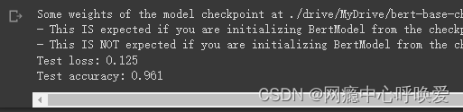
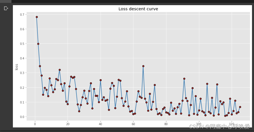
可以看到在测试集上的准确率到达了百分之96.1，并且没有过拟合的现象

模型预测

test_comments =  ['买的人很多，味道好，是十年以上的老店了']
predict(test_comments, model_config)
1
2

绘制loss曲线

import pandas as pd
import matplotlib.pyplot as plt

#设置绘图风格
plt.style.use('ggplot')
# 中文乱码的处理
plt.rcParams['font.sans-serif'] =['Microsoft YaHei']
plt.rcParams['axes.unicode_minus'] = False
#坐标轴负号的处理
plt.rcParams['axes.unicode_minus']=False
# 绘制单条折线图
plt.figure(figsize=(14,7))
plt.plot(train_loss_list_idx, # x轴数据
         train_loss_list, # y轴数据
         linestyle = '-', # 折线类型
         linewidth = 2, # 折线宽度
         color = 'steelblue', # 折线颜色
         marker = 'o', # 折线图中添加圆点
         markersize = 6, # 点的大小
         markeredgecolor='black', # 点的边框色
         markerfacecolor='brown', # 点的填充色
         )
# 添加y轴标签
plt.ylabel('loss')
# 添加图形标题
plt.title('Loss descent curve')
# 显示图形
plt.show()
1
2
3
4
5
6
7
8
9
10
11
12
13
14
15
16
17
18
19
20
21
22
23
24
25
26
27
28