r语言列表添加元素_学习 R 语言：快速开始

本文内容来自《R 语言编程艺术》(The Art of R Programming)，有部分修改

运行R

交互模式

使用命令行运行 R.exe (linux 中运行 R)

本文示例均在 Jupyter Lab 中运行 R 环境

注：在 Jupyter Notebook 中，只有使用 print 函数才能正确输出序号值， 直接执行变量名输出的结果没有序号，与 R 命令行交互环境中不同

下面代码为了展示输出结果均为向量，均使用 print 函数打印。如果直接在交互环境中运行，则不需要添加 print。

print(mean(abs(rnorm(100))))

[1] 0.7482577

print(rnorm(10))

 [1]  0.03721293 -0.20435474 -0.19896266 -0.81638471  2.38975757 -0.13099913 [7] -1.69019026  1.04377265  0.83753176 -1.41777840

批处理模式

pdf("xh.pdf")hist(rnorm(100))dev.off()

R.exe CMD BATCH z.R

R 会话

注：从本节开始，代码中省略 print 函数调用，与命令行交互模式保持一致

向量

R 语言中最基本的数据类型是向量

 是 R 语言的标准赋值运算符

使用 c 创建向量，c 表示连接 (concatenate)

x  c(1, 2, 4)x

[1] 1 2 4

c 中也可以使用向量，注意这种方式是将向量展开，而不是生成嵌套的向量

q  c(x, x, 8)q

[1] 1 2 4 1 2 4 8

注：对比 Python 列表的 append 和 expend 方法

访问向量中的元素

注意：R 语言中的索引从 1 开始！

与 C 语言和 Python 不同

x[3]

[1] 4

提取子集

注意：R 语言中的范围包含最后一个元素，即使用闭区间 [a, b]！

而 Python 中不包含最后一个元素，即使用左闭右开区间 [a, b)

x[2:3]

[1] 2 4

求统计值

求均值和标准差

mean(x)

[1] 2.333333

sd(x)

[1] 1.527525

将统计值赋值给变量

R 语言中的注释也以 # 开头

y  mean(x)y # print out y

[1] 2.333333

内置数据集

使用 data() 函数返回内置的数据集

data()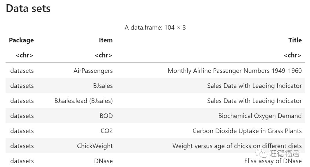

以尼罗河水流量数据集 Nile 为例，计算统计值

mean(Nile)

[1] 919.35

sd(Nile)

[1] 169.2275

画直方图

hist(Nile)

hist 提供各类参数来控制图形

例如，使用 breaks 函数指定分组数

hist(Nile, breaks=5)

调用 q() 函数可以退出 R 命令行交互模式。

函数入门

与 Python 类似，函数同样是 R 语言编程的核心

下面的函数统计向量中奇数的个数

其中 %% 是求余操作符(Python 中是 %)

oddcount  function(x) {    k  0for (n in x) {if (n %% 2 == 1) k  k + 1    }return(k)}

测试下上面的函数

oddcount(c(1, 3, 5))

[1] 3

oddcount(c(1, 2, 3, 7, 9))

[1] 4

变量的作用域

k 和 n 都是函数的局部变量。

参数 x 是形式参数 (formal argument)，R 语言中的形式参数是 局部变量。

函数内对参数的修改不会影响函数外的值。

注：这意味着函数调用会发生数据复制，需要考虑耗时问题。不知道是否有指针形式的参数传递方式？

函数可以访问全局变量

f  function(x) return(x+y)y  3f(5)

[1] 7.333333

注：上例可以看到 R 语言对函数变量的处理与 Python 类似，在实际执行时确定变量

函数内部给全局变量赋值需要使用超级赋值运算符 (superassignment operator) <，后续会介绍

默认函数

R 语言也支持默认参数

g  function(x, y=2, z=T) {return(z)}g(12, z=FALSE)

[1] FALSE

T 和 FALSE 都是布尔类型

重要数据结构

向量，R 语言中的战斗机

向量元素必须属于同一种模式 (mode)，或者说是数据类型

注意：R 语言中没有标量，单个数值是一元向量

x  8x

[1] 8

输出的 [1] 表示这行的开头是向量的第一个元素，也就意味着单个数被 R 语言当成长度为 1 的向量

字符串

字符串实际上是字符模式的单元素向量

先看数值模式的向量

x  c(5, 12, 13)x

[1]  5 12 13

length(x)

[1] 3

mode(x)

[1] "numeric"

创建字符串，即一元字符串向量

y  "abc"y

[1] "abc"

length(y)

[1] 1

mode(y)

[1] "numeric"

创建多元素字符串向量

z  c("abc", "29 88")length(z)

[1] 2

mode(z)

[1] "character"

字符串操作函数举例

u  paste("abc", "de", "f")print(u)

[1] "abc de f"

v  strsplit(u, " ")print(v)

[[1]][1] "abc" "de"  "f"

矩阵

矩阵是向量，附加两个属性：行数和列数

使用 rbind() 将多个向量逐行结合成一个矩阵

m  rbind(c(1, 4),c(2, 2))print(m)

     [,1] [,2][1,]    1    4[2,]    2    2

%*% 计算矩阵乘法

print(m %*% c(1, 1))

     [,1][1,]    5[2,]    4

矩阵使用双下标作为索引，与向量一样，索引从 1 开始

类似 Python 中 numpy 数组的索引方法

m[1, 2]

[1] 4

m[2, 2]

[1] 2

提取子矩阵

注：numpy 数组也提供类似的功能，不过 R 语言更简洁

print(m[1, ])  # 提取第 1 行

[1] 1 4

print(m[, 2])  # 提取第 2 列

[1] 4 2

列表

值的容器，各个元素可以属于不同的类型，使用名称来访问各元素。

注：类似 Python 中的字典 (dict)

x  list(u=2, v="abc")print(x)

$u[1] 2$v[1] "abc"

访问 u 组件

print(x$u)

[1] 2

列表常用于函数返回多个结果

上面调用 hist(Nile) 生成直方图，该函数也有返回值

hn  hist(Nile)

查看返回的内容，返回值描述了直方图的特征

hn

$breaks [1]  400  500  600  700  800  900 1000 1100 1200 1300 1400$counts [1]  1  0  5 20 25 19 12 11  6  1$density [1] 0.0001 0.0000 0.0005 0.0020 0.0025 0.0019 0.0012 0.0011 0.0006 0.0001$mids [1]  450  550  650  750  850  950 1050 1150 1250 1350$xname[1] "Nile"$equidist[1] TRUEattr(,"class")[1] "histogram"

也可以使用 str 函数以更简洁的方式打印列表，str 代表 structure

str(hn)

List of 6 $ breaks  : int [1:11] 400 500 600 700 800 900 1000 1100 1200 1300 ... $ counts  : int [1:10] 1 0 5 20 25 19 12 11 6 1 $ density : num [1:10] 0.0001 0 0.0005 0.002 0.0025 0.0019 0.0012 0.0011 0.0006 0.0001 $ mids    : num [1:10] 450 550 650 750 850 950 1050 1150 1250 1350 $ xname   : chr "Nile" $ equidist: logi TRUE - attr(*, "class")= chr "histogram"

数据框

Python 中大名鼎鼎的 pandas 库中核心概念 DataFrame 即来自 R 语言。

数据框可以当成是不同类型数据组成的“矩阵”。

数据框实际上的列表，只不过列表的每个组件是由“矩阵”数据的一列构成的。

d  data.frame(list(    kids=c("Jack", "Jill"),    ages=c(12, 10)))print(d)

  kids ages1 Jack   122 Jill   10

访问数据框的某列

print(d$ages)

[1] 12 10

类

简单介绍 S3 类的使用。

hist() 的返回值是一个列表，但还有一个属性 (attribute)，指定类表的类，这里是 histogram 类。

对 S3 类可以用 summary() 泛型函数查看摘要信息。

summary(hn)

         Length Class  Modebreaks   11     -none- numericcounts   10     -none- numericdensity  10     -none- numericmids     10     -none- numericxname     1     -none- characterequidist  1     -none- logical

扩展案例：考试成绩的回归分析

数据下载自 https://www.kaggle.com/dipam7/student-grade-prediction

原始数据来自 https://archive.ics.uci.edu/ml/datasets/student+performance

使用 read.csv 读取 CSV 文件

score  read.csv(file="student-mat.csv")

返回的结果是数据框类型

print(class(score))

[1] "data.frame"

使用 head 查看数据的前几行，因为 CSV 文件包含表头，所以数据列均已被命名

head(score)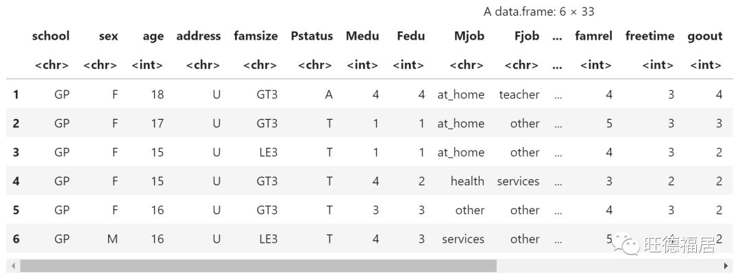

使用期中考试成绩 (G2) 预测期末考试成绩 (G3)

lm 函数实现线性拟合

lma  lm(score$G3 ~ score$G2)

lma 是 lm 类的一个实例。使用 attributes() 函数列出所有组件

print(attributes(lma))

$names [1] "coefficients"  "residuals"     "effects"       "rank" [5] "fitted.values" "assign"        "qr"            "df.residual" [9] "xlevels"       "call"          "terms"         "model"$class[1] "lm"

打印详细信息

str(lma)

List of 12 $ coefficients : Named num [1:2] -1.39 1.1  ..- attr(*, "names")= chr [1:2] "(Intercept)" "score$G2" $ residuals    : Named num [1:395] 0.78 1.882 2.576 0.963 0.372 ...  ..- attr(*, "names")= chr [1:395] "1" "2" "3" "4" ... $ effects      : Named num [1:395] -206.998 82.288 2.481 1.007 0.323 ...  ..- attr(*, "names")= chr [1:395] "(Intercept)" "score$G2" "" "" ... $ rank         : int 2 $ fitted.values: Named num [1:395] 5.22 4.12 7.42 14.04 9.63 ...  ..- attr(*, "names")= chr [1:395] "1" "2" "3" "4" ... $ assign       : int [1:2] 0 1 $ qr           :List of 5  ..$ qr   : num [1:395, 1:2] -19.8746 0.0503 0.0503 0.0503 0.0503 ...  .. ..- attr(*, "dimnames")=List of 2  .. .. ..$ : chr [1:395] "1" "2" "3" "4" ...  .. .. ..$ : chr [1:2] "(Intercept)" "score$G2"  .. ..- attr(*, "assign")= int [1:2] 0 1  ..$ qraux: num [1:2] 1.05 1.07  ..$ pivot: int [1:2] 1 2  ..$ tol  : num 1e-07  ..$ rank : int 2  ..- attr(*, "class")= chr "qr" $ df.residual  : int 393 $ xlevels      : Named list() $ call         : language lm(formula = score$G3 ~ score$G2) $ terms        :Classes 'terms', 'formula'  language score$G3 ~ score$G2  .. ..- attr(*, "variables")= language list(score$G3, score$G2)  .. ..- attr(*, "factors")= int [1:2, 1] 0 1  .. .. ..- attr(*, "dimnames")=List of 2  .. .. .. ..$ : chr [1:2] "score$G3" "score$G2"  .. .. .. ..$ : chr "score$G2"  .. ..- attr(*, "term.labels")= chr "score$G2"  .. ..- attr(*, "order")= int 1  .. ..- attr(*, "intercept")= int 1  .. ..- attr(*, "response")= int 1  .. ..- attr(*, ".Environment")=  .. ..- attr(*, "predvars")= language list(score$G3, score$G2)  .. ..- attr(*, "dataClasses")= Named chr [1:2] "numeric" "numeric"  .. .. ..- attr(*, "names")= chr [1:2] "score$G3" "score$G2" $ model        :'data.frame':	395 obs. of  2 variables:  ..$ score$G3: int [1:395] 6 6 10 15 10 15 11 6 19 15 ...  ..$ score$G2: int [1:395] 6 5 8 14 10 15 12 5 18 15 ...  ..- attr(*, "terms")=Classes 'terms', 'formula'  language score$G3 ~ score$G2  .. .. ..- attr(*, "variables")= language list(score$G3, score$G2)  .. .. ..- attr(*, "factors")= int [1:2, 1] 0 1  .. .. .. ..- attr(*, "dimnames")=List of 2  .. .. .. .. ..$ : chr [1:2] "score$G3" "score$G2"  .. .. .. .. ..$ : chr "score$G2"  .. .. ..- attr(*, "term.labels")= chr "score$G2"  .. .. ..- attr(*, "order")= int 1  .. .. ..- attr(*, "intercept")= int 1  .. .. ..- attr(*, "response")= int 1  .. .. ..- attr(*, ".Environment")=  .. .. ..- attr(*, "predvars")= language list(score$G3, score$G2)  .. .. ..- attr(*, "dataClasses")= Named chr [1:2] "numeric" "numeric"  .. .. .. ..- attr(*, "names")= chr [1:2] "score$G3" "score$G2" - attr(*, "class")= chr "lm"

组件名可以使用缩写，只要与其他名称不发生混淆即可。

注：作为当接触 R 的新人，笔者强烈不推荐使用缩写。太灵活会带来很多问题

当前代码自动补全已成为编辑器的标配，没有必要再使用缩写

例如，获取线性拟合的系数

print(lma$coef)

(Intercept)    score$G2  -1.392758    1.102112

直接打印 lma 展示的信息不多，实际上是调用 print.lm() 函数

print(lma)

Call:lm(formula = score$G3 ~ score$G2)Coefficients:(Intercept)     score$G2     -1.393        1.102

使用 summary() 可以展示更多信息，实际上是调用 summary.lm() 函数

summary(lma)

Call:lm(formula = score$G3 ~ score$G2)Residuals:    Min      1Q  Median      3Q     Max-9.6284 -0.3326  0.2695  1.0653  3.5759Coefficients:            Estimate Std. Error t value Pr(>|t|)(Intercept) -1.39276    0.29694   -4.69 3.77e-06 ***score$G2     1.10211    0.02615   42.14  < 2e-16 ***---Signif. codes:  0 '***' 0.001 '**' 0.01 '*' 0.05 '.' 0.1 ' ' 1Residual standard error: 1.953 on 393 degrees of freedomMultiple R-squared:  0.8188,	Adjusted R-squared:  0.8183F-statistic:  1776 on 1 and 393 DF,  p-value: < 2.2e-16

使用 G1 和 G2 成绩预测 G3 成绩

下面的 + 仅仅是预测变量 (predictor variable) 的分隔符

lmb  lm(score$G3 ~ score$G1 + score$G2)summary(lmb)

Call:lm(formula = score$G3 ~ score$G1 + score$G2)Residuals:    Min      1Q  Median      3Q     Max-9.5713 -0.3888  0.2885  0.9725  3.7089Coefficients:            Estimate Std. Error t value Pr(>|t|)(Intercept) -1.83001    0.33531  -5.458 8.57e-08 ***score$G1     0.15327    0.05618   2.728  0.00665 **score$G2     0.98687    0.04957  19.909  < 2e-16 ***---Signif. codes:  0 '***' 0.001 '**' 0.01 '*' 0.05 '.' 0.1 ' ' 1Residual standard error: 1.937 on 392 degrees of freedomMultiple R-squared:  0.8222,	Adjusted R-squared:  0.8213F-statistic: 906.1 on 2 and 392 DF,  p-value: < 2.2e-16

启动和关闭 R

R 会话启动时会执行保存在 .Rprofile 中的命令。

比如可以添加额外的库路径

.libPaths("/home/nm/R")

获取当前路径

current  getwd()print(current)

[1] "D:/windroc/project/study/r/tarp/chap01"

设置当前路径

setwd("D:/")getwd()setwd(current)getwd()

'D:/''D:/windroc/project/study/r/tarp/chap01'

获取帮助

help() 函数

help(seq)

? 可以快速调用 help() 函数

?seq

使用 help 时，特殊字符和一些保留字符必须用引号括起来

?"?"for"

example() 函数

example() 函数会运行示例代码

example(seq)

对于绘图函数，example 会提供图形化展示

example(persp)

搜索

如果不太清楚想要查找什么，可以使用 help.search() 函数进行查找

help.search("multivariate normal")

?? 是 help.search 快捷方法

??"multivariate normal"

其他主题的帮助

?mvrnorm

获取整个包的信息

help(package=MASS)

获得一般主题的帮助

?files

批处理模式的帮助

R CMD command --help

例如

R CMD install --help

互联网资源

Just Google it

---

题图由 Antonio López 在 Pixabay 上发布。