SLAM系列——视觉里程计（直接法）_视觉里程计直接法

1 直接法的引出

1. 特征点法的缺点：

   • 关键点的提取和描述子计算非常耗时
   • 使用特征点忽略了除特征点以外的其他信息
   • 相机可能运动到特征点缺失的地方，这些地方没有明显的纹理信息

2. 克服这些缺点的思路

   • 保留特征点，但是只计算关键点，不计算描述子，使用光流法（Optical Flow）来跟踪特征点的运动
   • 只计算关键点，不计算描述子，使用直接法（Direct Method）计算特征点在下一个时刻出现的位置。
   • 不计算关键字，也不计算描述子，根据像素灰度差异，直接计算相机运动

   第一种方法仍然使用特征点，只是把匹配描述子替换成光流跟踪，估计相机运动仍然使用对极几何、PnP或者ICP算法
   提取特征点，而在后两种中，会根据图像的像素灰度信息来计算相机运动，特闷都称为直接法

3. 特征点法和直接法区别：

   • 特征点法：最小化重投影误差（Reprojection Error）优化相机运动，需要精确地知道空间点在两个相机中投影后的像素位置，这也是需要匹配跟踪的原因，但是计算量大。
   • 直接法：不需要知道点和点的匹配关系，通过最小化光度误差（Photometric Error）
   4. 直接法根据 像素的亮度信息，估计相机的运动，可以完全不用计算关键点和描述子，于是，既避免了 特征的计算时间，也避免了特征缺失的情况。只要场景中存在明暗变化（可以是渐变，不形成局部的图像梯度），直接法就能工作。
   5. 根据使用像素的数量，直接法分为稀疏、稠密和 半稠密三种。相比于特征点法只能重构稀疏特征点（稀疏地图），直接法还具有恢复稠密或 半稠密结构的能力。

2 光流（Optical Flow)

1. 直接法是从光流演变而来的，光流描述了像素 在图像中的运动，而直接法则附带着一个相机运动模型。

（1）计算部分像素运动的稀疏光流
（2）计算所有像素运动的稠密光流

Lucas-Kanade光流

2. 引入 光流法的基本假设：

   灰度不变假设：同一个空间点的像素灰度值，在各个图像中是固定不变的。
   $$I(x+dx,y+dy,t+dt)=I(x,y,t)$$
   对左边进行泰勒一阶展开,保留一阶项
   $$I(x+dx,y+dy,t+dt)\approx I(x,y,t)+\frac{\partial I}{\partial x}dx+\frac{\partial I}{\partial y}dy+\frac{\partial I}{\partial t}dt$$
   $$\frac{\partial I}{\partial x}dx+\frac{\partial I}{\partial y}dy+\frac{\partial I}{\partial t}dt=0$$
   两边同时除以dt,得：
   $$\frac{\partial I}{\partial x}\frac{dx}{dt}+\frac{\partial I}{\partial y}\frac{dy}{dt}=-\frac{\partial I}{\partial t}$$
   dx/dt 为像素在 x 轴上运动速度，而 dy/dt 为 y 轴速度，把它们记为 u, v。同 时$\partial I/\partial x$为图像在该点处 x 方向的梯度，另一项则是在 y 方向的梯度，记为 $I_x,I_y$。图像灰度对时间的变化量记为 $I_t$,写成矩阵形式：
   $$\left[\begin{array}{cc}{I}_x& I_y\end{array}\right]\left[\begin{array}{c}u\\ v\end{array}\right]=-I_t$$

   运动相同假设：设某一个窗 口内的像素具有相同的运动。

   考虑一个大小ω∗ω窗口，含有${\omega }^2$个像素，得到${\omega }^2$个方程:
   $${\left[\begin{array}{cc}{I}_x& I_y\end{array}\right]}_k\left[\begin{array}{c}u\\ v\end{array}\right]=-I_{tk},k=1,2...,{\omega }^2.$$

记：
$$A=\left[\begin{array}{c}{\left[\begin{array}{cc}{I}_x& I_y\end{array}\right]}_1\\ ⋮\\ {\left[\begin{array}{cc}{I}_x& I_y\end{array}\right]}_k\end{array}\right],b=\left[\begin{array}{c}{I}_{t1}\\ ⋮\\ I_{tk}\end{array}\right]$$
整个方程为：
$$A\left[\begin{array}{c}u\\ v\end{array}\right]=-b$$
这是一个关于 u, v 的超定线性方程，传统解法是求最小二乘解
$${\left[\begin{array}{c}u\\ v\end{array}\right]}^{\ast }=-(A^{T}A{)}^{-1}{A}^{T}b$$
可以得到像素在图像间的运动$u,v$,由于像素梯度仅在局部有效，如果一次迭代不够好，会多次迭代。在SLAM中，LK光流长被用来估计角点的运动。

3 实践：LK光流

3.1 使用TMU公开数据集

3.2 使用LK光流

• 角点处稳定，边缘处会滑动，沿边缘移动时特征快的内容基本不变。
• 匹配描述子的方法在相机运动较大时仍能成功， 而光流必须要求相机运动是微小的。从这方面来说，光流的鲁棒性比描述子差一些。。
• LK光流跟踪能够直接得到特征点的对应关系，大多数只会碰到特征点跟丢，不太会遇到误匹配。
• 可以通过光流跟踪的特征点，用PnP、ICP或对极几何来估计相机运动。

#include <iostream>
#include <fstream>
#include <list>
#include <vector>
#include <chrono>
using namespace std; 

#include <opencv2/core/core.hpp>
#include <opencv2/highgui/highgui.hpp>
#include <opencv2/features2d/features2d.hpp>
#include <opencv2/video/tracking.hpp>

int main( int argc, char** argv )
{
//    if ( argc != 2 )
//    {
//        cout<<"usage: useLK path_to_dataset"<<endl;
//        return 1;
//    }
//    string path_to_dataset = argv[1];
//    string associate_file = path_to_dataset + "/associate.txt";
    string path_to_dataset ="/home/xiaohu//slambook-master/ch8/rgbd_dataset_freiburg1_desk";
    string associate_file = path_to_dataset+"/associate.txt";
    ifstream fin( associate_file );
    if ( !fin ) 
    {

        cerr<<"I cann't find associate.txt!"<<endl;
        return 1;
    }
    
    string rgb_file, depth_file, time_rgb, time_depth;
    list< cv::Point2f > keypoints;      // 因为要删除跟踪失败的点，使用list
    cv::Mat color, depth, last_color;
    
    for ( int index=0; index<100; index++ )
    {
        fin>>time_rgb>>rgb_file>>time_depth>>depth_file;
        color = cv::imread( path_to_dataset+"/"+rgb_file );
        depth = cv::imread( path_to_dataset+"/"+depth_file, -1 );
        if (index ==0 )
        {
            // 对第一帧提取FAST特征点
            vector<cv::KeyPoint> kps;
            cv::Ptr<cv::FastFeatureDetector> detector = cv::FastFeatureDetector::create();
            detector->detect( color, kps );
            for ( auto kp:kps )
                keypoints.push_back( kp.pt );
            last_color = color;
            continue;
        }
        if ( color.data==nullptr || depth.data==nullptr )
            continue;
        // 对其他帧用LK跟踪特征点
        vector<cv::Point2f> next_keypoints; 
        vector<cv::Point2f> prev_keypoints;
        for ( auto kp:keypoints )
            prev_keypoints.push_back(kp);
        vector<unsigned char> status;
        vector<float> error; 
        chrono::steady_clock::time_point t1 = chrono::steady_clock::now();
        cv::calcOpticalFlowPyrLK( last_color, color, prev_keypoints, next_keypoints, status, error );
        chrono::steady_clock::time_point t2 = chrono::steady_clock::now();
        chrono::duration<double> time_used = chrono::duration_cast<chrono::duration<double>>( t2-t1 );
        cout<<"LK Flow use time："<<time_used.count()<<" seconds."<<endl;
        // 把跟丢的点删掉
        int i=0; 
        for ( auto iter=keypoints.begin(); iter!=keypoints.end(); i++)
        {
            if ( status[i] == 0 )
            {
                iter = keypoints.erase(iter);
                continue;
            }
            *iter = next_keypoints[i];
            iter++;
        }
        cout<<"tracked keypoints: "<<keypoints.size()<<endl;
        if (keypoints.size() == 0)
        {
            cout<<"all keypoints are lost."<<endl;
            break; 
        }
        // 画出 keypoints
        cv::Mat img_show = color.clone();
        for ( auto kp:keypoints )
            cv::circle(img_show, kp, 10, cv::Scalar(0, 240, 0), 1);
        cv::imshow("corners", img_show);
        cv::waitKey(0);
        last_color = color;
    }
    return 0;
}
1
2
3
4
5
6
7
8
9
10
11
12
13
14
15
16
17
18
19
20
21
22
23
24
25
26
27
28
29
30
31
32
33
34
35
36
37
38
39
40
41
42
43
44
45
46
47
48
49
50
51
52
53
54
55
56
57
58
59
60
61
62
63
64
65
66
67
68
69
70
71
72
73
74
75
76
77
78
79
80
81
82
83
84
85
86
87
88
89
90
91
92
93

4 直接法

4.1 直接法的推导

记P的世界坐标为$[X,Y,Z]$,它在两个相机上成像，记非齐次像素坐标为$p_1$,$p_{12}$。
目标是求第一个相机到第二个相 机的相对位姿变换。我们以第一个相机为参照系，设第二个相机旋转和平移为 R, t（对应李代数为 ξ）。

$$p_1={\left[\begin{array}{c}u\\ v\\ 1\end{array}\right]}_1=\frac{1}{Z_1}KP$$
$$p_1={\left[\begin{array}{c}u\\ v\\ 1\end{array}\right]}_2=\frac{1}{Z_1}K(RP+t)=\frac{1}{Z_2}K(exp({\xi }^{\wedge })P{)}_{1:3}$$

特征点法中，通过匹配描述子，知道了 p1, p2 的像素位置，可以计 算重投影的位置。
直接法中，由于没有特征匹配，无从知道哪一个 p2 与 p1 对应着同一个点
直接法的思路是根据当前相机的位姿估计值，来寻找 p2 的位置。但若相机位姿不够好，p2 的外观和 p1 会有明显差别。于是，为了减小这个差别，我们优化相机的位姿，来寻找与 p1 更相似的 p2。这同样可以通过解一个优化问题，但此时最小化的不是重投影误差，而是光度误差，也就是 P 的两个像的亮度误差:

$$e=I_1\left(p_1\right)-I_2\left(p_2\right)$$
优化目标为该误差的二范数：
$$\underset{ϵ}{\min }J(\xi )={\Vert e\Vert }^2$$
仍是基于灰度不变假设，许多个（比如 N 个）空间点 $P_i$，那么，整 个相机位姿估计问题变为：
$$\underset{ϵ}{\min }J(\xi )=\sum _{i=1}^N{e}_i^T{e}_i,e_i=I_1(p_{1,i})-I_2(p_{2,i})$$
优化变量：相机位姿$\xi$,误差 e 是如何随着相机位姿 ξ 变化的，需要分析它们的导数关系,因此，使用李代数上的扰动模型。我 们给 $exp(\xi )$ 左乘一个小扰动 $exp(\delta \xi )$，得：

q 为 P 在扰动之后，位于第二个相机坐标系下的坐标，而 u 为它的像素坐标。利用一阶泰勒展开，有：

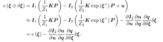
1. ∂I2/∂u 为 u 处的像素梯度；
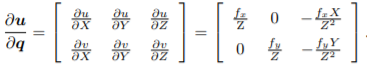
2. ∂u/∂q 为投影方程关于相机坐标系下的三维点的导数。记$q=[X,Y,Z]$
   
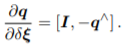
3. ∂q/∂δξ 为变换后的三维点对变换的导数
   后两项合并:
   
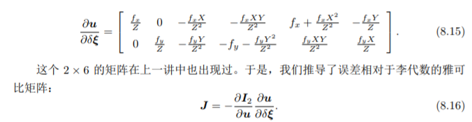
   对于 N 个点的问题，我们可以用这种方法计算优化问题的雅可比矩阵，然后使用 高斯牛顿法或列文伯格——马夸尔特方法计算增量，迭代求解。

4.2 直接法的讨论

在上面的推导中，P是一个已知位置的空间点，在RGB-D相机下，我们可以把任意像素反投影到三维空间，然后投影到下一个图像中。如果在单目相机中，可以使用已经估计好位置的特征点（虽然是特征点，但直接法里是可以避免计算描述子的）。根据P的来源，把直接法进行分类：

• P来自于稀疏特征点，称之为稀疏直接法。通常我们使用数百个特征点，并且会像L-K光流那样，假设它周围像素也是不变的。这种稀疏直接法速度不必计算描述子，并且只使用数百个像素，因此速度最快，但只能计算稀疏的重构。
• P来自部分像素, 这称之为半稠密（Semi-Dense）的直接法，考虑只使用带有梯度的像素点，舍弃像素梯度不明显的地方，可以重构一个半稠密结构。
• P为所有像素，称为稠密直接法。稠密重构需要计算所有像素（一般几十万至几百万个），因此多数不能在现有的 CPU上实时计算，需要GPU的加速。

可以看到，从稀疏到稠密重构，都可以用直接法来计算。它们的计算量是逐渐增长的。稀疏方法可以快速地求解相机位姿，而稠密方法可以建立完整地图。

5 实践：RGB-D的直接法

图优化：误差项为单个像素的光度误差。由于 g2o 中本身没有计算光度误差的边，我们需要 自己定义一种新的边。在上述的建模中，直接法图优化问题是由一个相机位姿顶点与许多条一元边组成的。

5.1 稀梳直接法

#include <iostream>
#include <fstream>
#include <list>
#include <vector>
#include <chrono>
#include <ctime>
#include <climits>

#include <opencv2/core/core.hpp>
#include <opencv2/imgproc/imgproc.hpp>
#include <opencv2/highgui/highgui.hpp>
#include <opencv2/features2d/features2d.hpp>

#include <g2o/core/base_unary_edge.h>
#include <g2o/core/block_solver.h>
#include <g2o/core/optimization_algorithm_levenberg.h>
#include <g2o/solvers/dense/linear_solver_dense.h>
#include <g2o/core/robust_kernel.h>
#include <g2o/types/sba/types_six_dof_expmap.h>

using namespace std;
using namespace g2o;

/********************************************
* 本节演示了RGBD上的稀疏直接法 
********************************************/

// 一次测量的值，包括一个世界坐标系下三维点与一个灰度值
struct Measurement
{
   Measurement ( Eigen::Vector3d p, float g ) : pos_world ( p ), grayscale ( g ) {}
   Eigen::Vector3d pos_world;
   float grayscale;
};

inline Eigen::Vector3d project2Dto3D ( int x, int y, int d, float fx, float fy, float cx, float cy, float scale )
{
   float zz = float ( d ) /scale;
   float xx = zz* ( x-cx ) /fx;
   float yy = zz* ( y-cy ) /fy;
   return Eigen::Vector3d ( xx, yy, zz );
}

inline Eigen::Vector2d project3Dto2D ( float x, float y, float z, float fx, float fy, float cx, float cy )
{
   float u = fx*x/z+cx;
   float v = fy*y/z+cy;
   return Eigen::Vector2d ( u,v );
}

// 直接法估计位姿
// 输入：测量值（空间点的灰度），新的灰度图，相机内参； 输出：相机位姿
// 返回：true为成功，false失败
bool poseEstimationDirect ( const vector<Measurement>& measurements, cv::Mat* gray, Eigen::Matrix3f& intrinsics, Eigen::Isometry3d& Tcw );


// project a 3d point into an image plane, the error is photometric error
// an unary edge with one vertex SE3Expmap (the pose of camera)
class EdgeSE3ProjectDirect: public BaseUnaryEdge< 1, double, VertexSE3Expmap>
{
public:
   EIGEN_MAKE_ALIGNED_OPERATOR_NEW

   EdgeSE3ProjectDirect() {}

   EdgeSE3ProjectDirect ( Eigen::Vector3d point, float fx, float fy, float cx, float cy, cv::Mat* image )
       : x_world_ ( point ), fx_ ( fx ), fy_ ( fy ), cx_ ( cx ), cy_ ( cy ), image_ ( image )
   {}

   virtual void computeError()
   {
       const VertexSE3Expmap* v  =static_cast<const VertexSE3Expmap*> ( _vertices[0] );
       //.map函数，它的功能是把世界坐标系下三维点变换到相机坐标系，函数在g2o/types/sim3/sim3.h
       Eigen::Vector3d x_local = v->estimate().map ( x_world_ );
       float x = x_local[0]*fx_/x_local[2] + cx_;
       float y = x_local[1]*fy_/x_local[2] + cy_;
       // check x,y is in the image
       if ( x-4<0 || ( x+4 ) >image_->cols || ( y-4 ) <0 || ( y+4 ) >image_->rows )
       {
           _error ( 0,0 ) = 0.0;
           this->setLevel ( 1 );
       }
       else
       {
           _error ( 0,0 ) = getPixelValue ( x,y ) - _measurement;
       }
   }

   // plus in manifold
   virtual void linearizeOplus( )
   {
       if ( level() == 1 )
       {
           _jacobianOplusXi = Eigen::Matrix<double, 1, 6>::Zero();
           return;
       }
       VertexSE3Expmap* vtx = static_cast<VertexSE3Expmap*> ( _vertices[0] );
       Eigen::Vector3d xyz_trans = vtx->estimate().map ( x_world_ );   // q in book

       double x = xyz_trans[0];
       double y = xyz_trans[1];
       double invz = 1.0/xyz_trans[2];
       double invz_2 = invz*invz;

       float u = x*fx_*invz + cx_;
       float v = y*fy_*invz + cy_;

       // jacobian from se3 to u,v
       // NOTE that in g2o the Lie algebra is (\omega, \epsilon), where \omega is so(3) and \epsilon the translation
       Eigen::Matrix<double, 2, 6> jacobian_uv_ksai;
       //旋转在前，平移在后
       jacobian_uv_ksai ( 0,0 ) = - x*y*invz_2 *fx_;
       jacobian_uv_ksai ( 0,1 ) = ( 1+ ( x*x*invz_2 ) ) *fx_;
       jacobian_uv_ksai ( 0,2 ) = - y*invz *fx_;
       jacobian_uv_ksai ( 0,3 ) = invz *fx_;
       jacobian_uv_ksai ( 0,4 ) = 0;
       jacobian_uv_ksai ( 0,5 ) = -x*invz_2 *fx_;

       jacobian_uv_ksai ( 1,0 ) = - ( 1+y*y*invz_2 ) *fy_;
       jacobian_uv_ksai ( 1,1 ) = x*y*invz_2 *fy_;
       jacobian_uv_ksai ( 1,2 ) = x*invz *fy_;
       jacobian_uv_ksai ( 1,3 ) = 0;
       jacobian_uv_ksai ( 1,4 ) = invz *fy_;
       jacobian_uv_ksai ( 1,5 ) = -y*invz_2 *fy_;

       Eigen::Matrix<double, 1, 2> jacobian_pixel_uv;

       jacobian_pixel_uv ( 0,0 ) = ( getPixelValue ( u+1,v )-getPixelValue ( u-1,v ) ) /2;
       jacobian_pixel_uv ( 0,1 ) = ( getPixelValue ( u,v+1 )-getPixelValue ( u,v-1 ) ) /2;

       _jacobianOplusXi = jacobian_pixel_uv*jacobian_uv_ksai;
   }

   // dummy read and write functions because we don't care...
   virtual bool read ( std::istream& in ) {}
   virtual bool write ( std::ostream& out ) const {}

protected:
   // get a gray scale value from reference image (bilinear interpolated)
   inline float getPixelValue ( float x, float y )
   {
       //双线性插值通过寻找距离这个对应坐标最近的四个像素点，来计算该点的值（灰度值或者RGB值）。
       uchar* data = & image_->data[ int ( y ) * image_->step + int ( x ) ];
       float xx = x - floor ( x );
       float yy = y - floor ( y );
       return float (
                  ( 1-xx ) * ( 1-yy ) * data[0] +
                  xx* ( 1-yy ) * data[1] +
                  ( 1-xx ) *yy*data[ image_->step ] +
                  xx*yy*data[image_->step+1]
              );
   }
public:
   Eigen::Vector3d x_world_;   // 3D point in world frame
   float cx_=0, cy_=0, fx_=0, fy_=0; // Camera intrinsics
   cv::Mat* image_=nullptr;    // reference image
};

int main ( int argc, char** argv )
{
//    if ( argc != 2 )
//    {
//        cout<<"usage: useLK path_to_dataset"<<endl;
//        return 1;
//    }
   srand ( ( unsigned int ) time ( 0 ) );
//    string path_to_dataset = argv[1];
   string path_to_dataset ="/home/xiaohu//slambook-master/ch8/rgbd_dataset_freiburg1_desk";
   string associate_file = path_to_dataset + "/associate.txt";

   ifstream fin ( associate_file );

   string rgb_file, depth_file, time_rgb, time_depth;
   cv::Mat color, depth, gray;
   vector<Measurement> measurements;
   // 相机内参
   float cx = 325.5;
   float cy = 253.5;
   float fx = 518.0;
   float fy = 519.0;
   float depth_scale = 1000.0;
   Eigen::Matrix3f K;
   K<<fx,0.f,cx,0.f,fy,cy,0.f,0.f,1.0f;

   Eigen::Isometry3d Tcw = Eigen::Isometry3d::Identity();

   cv::Mat prev_color;
   // 我们以第一个图像为参考，对后续图像和参考图像做直接法
   for ( int index=0; index<10; index++ )
   {
       cout<<"*********** loop "<<index<<" ************"<<endl;
       fin>>time_rgb>>rgb_file>>time_depth>>depth_file;
       color = cv::imread ( path_to_dataset+"/"+rgb_file );
       depth = cv::imread ( path_to_dataset+"/"+depth_file, -1 );
       if ( color.data==nullptr || depth.data==nullptr )
           continue; 
       cv::cvtColor ( color, gray, cv::COLOR_BGR2GRAY );
       if ( index ==0 )
       {
           // 对第一帧提取FAST特征点
           vector<cv::KeyPoint> keypoints;
           cv::Ptr<cv::FastFeatureDetector> detector = cv::FastFeatureDetector::create();
           detector->detect ( color, keypoints );
           for ( auto kp:keypoints )
           {
               // 去掉邻近边缘处的点
               if ( kp.pt.x < 20 || kp.pt.y < 20 || ( kp.pt.x+20 ) >color.cols || ( kp.pt.y+20 ) >color.rows )
                   continue;
               ushort d = depth.ptr<ushort> ( cvRound ( kp.pt.y ) ) [ cvRound ( kp.pt.x ) ];
               if ( d==0 )
                   continue;
               Eigen::Vector3d p3d = project2Dto3D ( kp.pt.x, kp.pt.y, d, fx, fy, cx, cy, depth_scale );
               float grayscale = float ( gray.ptr<uchar> ( cvRound ( kp.pt.y ) ) [ cvRound ( kp.pt.x ) ] );
               measurements.push_back ( Measurement ( p3d, grayscale ) );
           }
           prev_color = color.clone();
           continue;
       }
       // 使用直接法计算相机运动
       chrono::steady_clock::time_point t1 = chrono::steady_clock::now();
       poseEstimationDirect ( measurements, &gray, K, Tcw );
       chrono::steady_clock::time_point t2 = chrono::steady_clock::now();
       chrono::duration<double> time_used = chrono::duration_cast<chrono::duration<double>> ( t2-t1 );
       cout<<"direct method costs time: "<<time_used.count() <<" seconds."<<endl;
       cout<<"Tcw="<<Tcw.matrix() <<endl;

       // plot the feature points
       cv::Mat img_show ( color.rows*2, color.cols, CV_8UC3 );
       prev_color.copyTo ( img_show ( cv::Rect ( 0,0,color.cols, color.rows ) ) );
       color.copyTo ( img_show ( cv::Rect ( 0,color.rows,color.cols, color.rows ) ) );
       for ( Measurement m:measurements )
       {
           //任何一次对 rand 的调用，都将得到一个 0~RAND_MAX 之间的伪随机数。
           if ( rand() > RAND_MAX/5 )
               continue;
           Eigen::Vector3d p = m.pos_world;
           Eigen::Vector2d pixel_prev = project3Dto2D ( p ( 0,0 ), p ( 1,0 ), p ( 2,0 ), fx, fy, cx, cy );
           Eigen::Vector3d p2 = Tcw*m.pos_world;
           Eigen::Vector2d pixel_now = project3Dto2D ( p2 ( 0,0 ), p2 ( 1,0 ), p2 ( 2,0 ), fx, fy, cx, cy );
           if ( pixel_now(0,0)<0 || pixel_now(0,0)>=color.cols || pixel_now(1,0)<0 || pixel_now(1,0)>=color.rows )
               continue;

           float b = 255*float ( rand() ) /RAND_MAX;
           float g = 255*float ( rand() ) /RAND_MAX;
           float r = 255*float ( rand() ) /RAND_MAX;
           cv::circle ( img_show, cv::Point2d ( pixel_prev ( 0,0 ), pixel_prev ( 1,0 ) ), 8, cv::Scalar ( b,g,r ), 2 );
           cv::circle ( img_show, cv::Point2d ( pixel_now ( 0,0 ), pixel_now ( 1,0 ) +color.rows ), 8, cv::Scalar ( b,g,r ), 2 );
           cv::line ( img_show, cv::Point2d ( pixel_prev ( 0,0 ), pixel_prev ( 1,0 ) ), cv::Point2d ( pixel_now ( 0,0 ), pixel_now ( 1,0 ) +color.rows ), cv::Scalar ( b,g,r ), 1 );
       }
       cv::imshow ( "result", img_show );
       cv::waitKey ( 0 );

   }
   return 0;
}

bool poseEstimationDirect ( const vector< Measurement >& measurements, cv::Mat* gray, Eigen::Matrix3f& K, Eigen::Isometry3d& Tcw )
{
   // 初始化g2o
   typedef g2o::BlockSolver<g2o::BlockSolverTraits<6,1>> DirectBlock;  // 求解的向量是6＊1的
   DirectBlock::LinearSolverType* linearSolver = new g2o::LinearSolverDense< DirectBlock::PoseMatrixType > ();
   DirectBlock* solver_ptr = new DirectBlock ( linearSolver );
   // g2o::OptimizationAlgorithmGaussNewton* solver = new g2o::OptimizationAlgorithmGaussNewton( solver_ptr ); // G-N
   g2o::OptimizationAlgorithmLevenberg* solver = new g2o::OptimizationAlgorithmLevenberg ( solver_ptr ); // L-M
   g2o::SparseOptimizer optimizer;
   optimizer.setAlgorithm ( solver );
   optimizer.setVerbose( true );

   g2o::VertexSE3Expmap* pose = new g2o::VertexSE3Expmap();
   pose->setEstimate ( g2o::SE3Quat ( Tcw.rotation(), Tcw.translation() ) );
   pose->setId ( 0 );
   optimizer.addVertex ( pose );

   // 添加边
   int id=1;
   for ( Measurement m: measurements )
   {
       EdgeSE3ProjectDirect* edge = new EdgeSE3ProjectDirect (
           m.pos_world,
           K ( 0,0 ), K ( 1,1 ), K ( 0,2 ), K ( 1,2 ), gray
       );
       edge->setVertex ( 0, pose );
       edge->setMeasurement ( m.grayscale );
       edge->setInformation ( Eigen::Matrix<double,1,1>::Identity() );
       edge->setId ( id++ );
       optimizer.addEdge ( edge );
   }
   cout<<"edges in graph: "<<optimizer.edges().size() <<endl;
   optimizer.initializeOptimization();
   optimizer.optimize ( 30 );
   Tcw = pose->estimate();
}


1
2
3
4
5
6
7
8
9
10
11
12
13
14
15
16
17
18
19
20
21
22
23
24
25
26
27
28
29
30
31
32
33
34
35
36
37
38
39
40
41
42
43
44
45
46
47
48
49
50
51
52
53
54
55
56
57
58
59
60
61
62
63
64
65
66
67
68
69
70
71
72
73
74
75
76
77
78
79
80
81
82
83
84
85
86
87
88
89
90
91
92
93
94
95
96
97
98
99
100
101
102
103
104
105
106
107
108
109
110
111
112
113
114
115
116
117
118
119
120
121
122
123
124
125
126
127
128
129
130
131
132
133
134
135
136
137
138
139
140
141
142
143
144
145
146
147
148
149
150
151
152
153
154
155
156
157
158
159
160
161
162
163
164
165
166
167
168
169
170
171
172
173
174
175
176
177
178
179
180
181
182
183
184
185
186
187
188
189
190
191
192
193
194
195
196
197
198
199
200
201
202
203
204
205
206
207
208
209
210
211
212
213
214
215
216
217
218
219
220
221
222
223
224
225
226
227
228
229
230
231
232
233
234
235
236
237
238
239
240
241
242
243
244
245
246
247
248
249
250
251
252
253
254
255
256
257
258
259
260
261
262
263
264
265
266
267
268
269
270
271
272
273
274
275
276
277
278
279
280
281
282
283
284
285
286
287
288
289
290
291
292
293
294

5.4 半稠密直接法

// select the pixels with high gradiants 
for ( int x=10; x<gray.cols-10; x++ )
    for ( int y=10; y<gray.rows-10; y++ )
    {
        Eigen::Vector2d delta (
            gray.ptr<uchar>(y)[x+1] - gray.ptr<uchar>(y)[x-1], 
            gray.ptr<uchar>(y+1)[x] - gray.ptr<uchar>(y-1)[x]
        );
        if ( delta.norm() < 50 )
            continue;
        ushort d = depth.ptr<ushort> (y)[x];
        if ( d==0 )
            continue;
        Eigen::Vector3d p3d = project2Dto3D ( x, y, d, fx, fy, cx, cy, depth_scale );
        float grayscale = float ( gray.ptr<uchar> (y) [x] );
        measurements.push_back ( Measurement ( p3d, grayscale ) );
    }
1
2
3
4
5
6
7
8
9
10
11
12
13
14
15
16
17

5.5 直接法的讨论

1. 相比于特征点法，直接法完全依靠优化来求解相机位姿,像 素梯度引导着优化的方向。如果我们想要得到正确的优化结果，就必须保证大部分像素梯 度能够把优化引导到正确的方向。

2. 在非线性优化过程中，这个位姿是由一个初值不断地优化迭代得到的（可以大致赋值初值），我们的初值比较差。

3. 直接法的梯度是直接由图像梯度确定的，因此我们必须保证沿着图像梯度走时，灰度误差会不断下降。然而，图像通常是一个很强烈的非凸函数。实际当中， 如果我们沿着图像梯度前进，很容易由于图像本身的非凸性（或噪声）落进一个局部极小值中，无法继续优化。只有当相机运动很小，图像中的梯度不会有很强的非凸性时，直接法才能成立。

5.6 直接法的优缺点总结

1. 优点：

   • 可以省去计算特征点、描述子的时间。
   • 只要求有像素梯度即可，无须特征点。因此，直接法可以在特征缺失的场合下使用。
   • 可以构建半稠密乃至稠密的地图，这是特征点法无法做到的。

2. 缺点：

   • 非凸性。直接法完全依靠梯度搜索，降低目标函数来计算相机位姿。其目标函数中需要取像素点的灰度值，而图像是强烈非凸的函数。这使得优化算法容易进入极小，只在运动很小时直接法才能成功。
   • 单个像素没有区分度。找一个和他像的实在太多了！——于是我们要么计算图像块，要么计算复杂的相关性。由于每个像素对改变相机运动的“意见”不一致。只能少数服从多数，以数量代替质量。
   • 灰度值不变是很强的假设。如果相机是自动曝光的，当它调整曝光参数时，会使得图像整体变亮或变暗。光照变化时亦会出现这种情况。特征点法对光照具有一定的容忍性，而直接法由于计算灰度间的差异，整体灰度变化会破坏灰度不变假设，使算法失败。