计算机视觉——多视图几何_多视角几何

1.前言

1.1 多视图几何概念

多视图几何是利用在不同视点所拍摄图像间的关系，来研究照相机之间或者特征之间关系的一门科学。

多视图几何（Multiple View Geometry）多视图几何主要研究用几何的方法，通过若干幅二维图像，来恢复三维物体。换言之就是研究三维重构，主要应用与计算机视觉中。

三维重构，即如何从静止物体不同视点下的图像中恢复物体三维几何结构信息。

在三维重构的过程中摄像机标定是一个极其重要环节，摄像机标定的研究分为三个部分：
（1）基于场景结构信息的标定；
（2）基于摄像机主动信息（纯旋转）的自标定；
（3）不依赖场景结构和摄像机主动信息的自标定。

2. 基本原理

2.1 对极几何

对极几何（Epipolar Geometry）描述的是两幅视图之间的内在射影关系，与外部场景无关，只依赖于摄像机内参数和这两幅试图之间的的相对姿态。

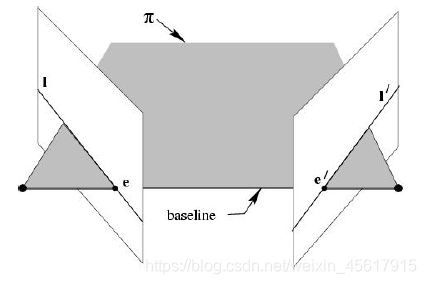
如下图所示，X为空间中的一点，x和x’为X在不同像平面中的投影，其中X与C, C’, x, x’ 共面。

tips：如果知道空间中点X在一幅图像中的投影点x，是无法确定空间中点X的位置以及X在其他图像中的投影点。

这里可以明确如下概念：

对极平面束（epipolar pencil）：以基线为轴的平面束；下图给出了包含两个平面的对极平面束。

对极平面（epipolar plane）：任何包含基线的平面都称为对极平面，或者说是对极平面束中的平面；例如，下图中的平面π就是一个对极平面。

对极点（epipole）：摄像机的基线与每幅图像的交点；即下图中的点e和e’。

对极线（epipolar line）：对极平面与图像的交线；例如，上图中的直线l和l’。

点x、x’与摄像机中心C和C’是共面的，并且与空间点X也是共面的，这5个点共面于平面π，这是一个最本质的约束，即5个点决定了一个平面π。

由该约束，可以推导出一个重要性质：由图像点x和x’反投影的射线共面，并且，在平面π上。 在搜索点对应中，该性质非常重要
由此引出基础矩阵的概念。

2.2 基础矩阵

2.2.1 基础矩阵推导

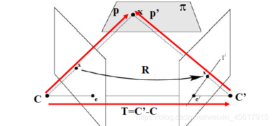
如上图所示，设X分别以C,C’为坐标原点，x的坐标被表示为p和p’，则有
$$p=R{p}^{\prime }+T$$
其中R、T表示在两个坐标系之间的旋转和位移。
在以C为坐标系原点的时候有：$x=Kp\Rightarrow p=K^{-1}x$
在以C’为坐标系原点的时候有：$x^{\prime }=K^{\prime }{p}^{\prime }\Rightarrow p^{\prime }=K^{\prime -1}{x}^{\prime }$
根据三点共面的性质可以知道：
$$(p-T{)}^T(T\times p)=0$$
又因为$$p=R{p}^{\prime }+T$$得到$$p-T=R{p}^{\prime }$$，所以上式可化简如下：
$$(R^T{p}^{\prime }{)}^T(T\times p)=0$$
其中$T\times p=Sp$，又 S = [ 0 − T z T y T z 0 − T x − T y T x 0 ] S=

$$\begin{bmatrix} 0& -T_z & T_y\\ T_z& 0 &-T_x \\ -T_y& T_x & 0 \end{bmatrix}$$ S=⎣⎡​0Tz​−Ty​​−Tz​0Tx​​Ty​−Tx​0​⎦⎤​
所以$$(R^T{p}^{\prime }{)}^T(T\times p)=0$$可写为下式：
$$(R^T{p}^{\prime }{)}^T(Sp)=0\Rightarrow (p^{\prime T}R)(Sp)=0\Rightarrow p^{\prime T}Ep=0$$
最终得到的如上式为本质矩阵。本质矩阵描述了空间中的点X在两个坐标系中的坐标对应关系。

根据上一篇博客中提到的$K$和$K^{\prime }$分别为两个相机的内参矩阵，有：
$p=K^{-1}x{p}^{\prime }=K^{\prime -1}{x}^{\prime }$
用上式代替 $p^{\prime T}Ep=0$ 中的p和p’ 可以得到下式：
$$(K^{-1}x{)}^{T}E(K^{\prime -1}{x}^{\prime })=0$$

$$\Rightarrow x^{\prime T}{K}^{-T}E{K}^{-1}x=0$$

$$\Rightarrow x^{\prime T}Fx=0$$
经推到得到了上述基础矩阵$F$,基础矩阵描述了空间中的点在两个像平面中的坐标对应关系。

注意：
分别以C,C’为坐标原点，x的坐标被表示为p和p’，则有下式：
$$p^{\prime T}Ep=0$$
其实E表示p’和p之间的位置关系，E为本质矩阵。

2.2.2 求解基础矩阵

基本矩阵是由下述方程定义：
$$x^{\prime T}Fx=0$$
其中$x\leftrightarrow x^{\prime }x\leftrightarrow x\prime$是两幅图像的任意一对匹配点。由于每一组点的匹配提供了计算$F$系数的一个线性方程，当给定至少7个点（3×3的齐次矩阵减去一个尺度，以及一个秩为2的约束），方程就可以计算出未知的$F$。
记点的坐标为$x=(x,y,1{)}^T，x^{\prime }=(x^{\prime },y^{\prime },1{)}^T，$则对应的方程为:
[ x x 1 ] [ f 11 f 12 f 13 f 21 f 22 f 23 f 31 f 32 f 33 ] [ x ′ y ′ 1 ] = 0

$$\begin{bmatrix} x& x& 1 \end{bmatrix}$$ $$\begin{bmatrix} f_{11}& f_{12}& f_{13}\\ f_{21}& f_{22}& f_{23}\\ f_{31}& f_{32}& f_{33}\\ \end{bmatrix}$$ $$\begin{bmatrix} x'\\ y'\\ 1 \end{bmatrix}$$ =0 [x​x​1​]⎣⎡​f11​f21​f31​​f12​f22​f32​​f13​f23​f33​​⎦⎤​⎣⎡​x′y′1​⎦⎤​=0
展开后有：
$$x^{\prime }x{f}_{11}+x^{\prime }y{f}_{12}+x^{\prime }{f}_{13}+y^{\prime }x{f}_{21}+y^{\prime }y{f}_{22}+y^{\prime }{f}_{23}+x{f}_{31}+y{f}_{32}+f_{33}=0$$
把矩阵$F$写成列向量的形式，则有：
$$[x^{\prime }x{x}^{\prime }y{x}^{\prime }{y}^{\prime }x{y}^{\prime }y{y}^{\prime }xy1]f=0$$
给定$n$组点的集合，我们有如下方程：
$$Af=\left[\begin{array}{ccccccccc}{x}_1^{\prime }{x}_1& x_1^{\prime }{y}_1& x_1^{\prime }& y_1^{\prime }{x}_1& y_1^{\prime }{y}_1& y_1^{\prime }& x_1& y_1& 1\\ ⋮& ⋮& ⋮& ⋮& ⋮& ⋮& ⋮& ⋮& ⋮\\ x_n^{\prime }{x}_n& x_n^{\prime }{y}_n& x_n^{\prime }& y_n^{\prime }{x}_n& y_n^{\prime }{y}_n& y_n^{\prime }& x_n& y_n& 1\end{array}\right]f=0$$

如果存在确定（非零）解，则系数矩阵$A$的秩最多是$8$。由于F是齐次矩阵，所以如果矩阵$A$的秩为$8$，则在差一个尺度因子的情况下解是唯一的。可以直接用线性算法解得。

如果由于点坐标存在噪声则矩阵$A$的秩可能大于$8$（也就是等于$9$，由于$A$是$n\ast 9$的矩阵）。这时候就需要求最小二乘解，这里就可以用SVD来求解，ff的解就是系数矩阵$A$最小奇异值对应的奇异向量，也就是$A$奇异值分解后$A=UD{V}^T$
中矩阵$V$的最后一列矢量，这是在解矢量$f$在约束$\Vert f\Vert$下取$\Vert Af\Vert$最小的解。

求解基础矩阵可分为如下两步：

1. 求线性解。由系数矩阵$A$最小奇异值对应的奇异矢量$f$求的$F$。
2. 奇异性约束。是最小化Frobenius范数$\Vert F-F^{\prime }\Vert$的F’代替F。

8点求解基础矩阵算法是计算基本矩阵的最简单的方法。为了提高解的稳定性和精度，往往会对输入点集的坐标先进行归一化处理。

3. 实验过程

3.1 实验数据准备

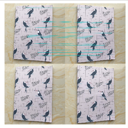
在本次实验中，拍摄三组不同的图像来求解基础矩阵并且观察极线的分布，数据如下：
第一组数据：左右拍摄，极点位于图像平面上（左右拍摄）

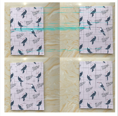
第二组数据：像平面接近平行，极点位于无穷远（左右平移）

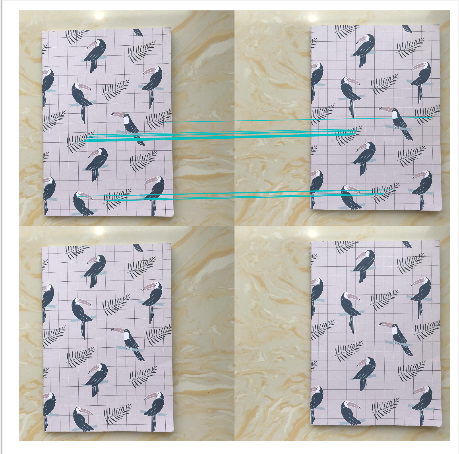
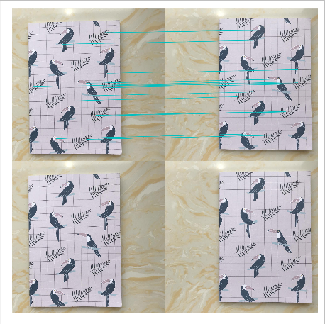
第三组数据：图像拍摄位置位于前后（远近不同）

3.2 基础矩阵的计算

关于基础矩阵的计算，本次实验设计7点、8点、10点计算基础矩阵，对于匹配点的个数对于基础矩阵的结果有何影响。

3.2.1 实验代码

from PIL import Image
from numpy import *
from pylab import *
import numpy as np
from PCV.geometry import camera
from PCV.geometry import homography
from PCV.geometry import sfm
from PCV.localdescriptors import sift
# Read features
# 载入图像，并计算特征
im1 = array(Image.open('data/5.jpg'))
sift.process_image('data/5.jpg', 'im5.sift')
l1, d1 = sift.read_features_from_file('im5.sift')
im2 = array(Image.open('data/6.jpg'))
sift.process_image('data/6.jpg', 'im6.sift')
l2, d2 = sift.read_features_from_file('im6.sift')
# 匹配特征
matches = sift.match_twosided(d1, d2)
ndx = matches.nonzero()[0]
# 使用齐次坐标表示，并使用 inv(K) 归一化
x1 = homography.make_homog(l1[ndx, :2].T)
ndx2 = [int(matches[i]) for i in ndx]
x2 = homography.make_homog(l2[ndx2, :2].T)
x1n = x1.copy()
x2n = x2.copy()
print(len(ndx))
figure(figsize=(16,16))
sift.plot_matches(im1, im2, l1, l2, matches, True)
show()
# Don't use K1, and K2
#def F_from_ransac(x1, x2, model, maxiter=5000, match_threshold=1e-6):
def F_from_ransac(x1, x2, model, maxiter=5000, match_threshold=1e-6):
    """ Robust estimation of a fundamental matrix F from point
    correspondences using RANSAC (ransac.py from
    http://www.scipy.org/Cookbook/RANSAC).
    input: x1, x2 (3*n arrays) points in hom. coordinates. """
    from PCV.tools import ransac
    data = np.vstack((x1, x2))
    d = 20 # 20 is the original
    # compute F and return with inlier index
    F, ransac_data = ransac.ransac(data.T, model,8, maxiter, match_threshold, d, return_all=True)
    return F, ransac_data['inliers']
# find E through RANSAC
# 使用 RANSAC 方法估计 E
model = sfm.RansacModel()
F, inliers = F_from_ransac(x1n, x2n, model, maxiter=5000, match_threshold=1e-4)
print(len(x1n[0]))
print(len(inliers))
# 计算照相机矩阵（P2 是 4 个解的列表）
P1 = array([[1, 0, 0, 0], [0, 1, 0, 0], [0, 0, 1, 0]])
P2 = sfm.compute_P_from_fundamental(F)
# triangulate inliers and remove points not in front of both cameras
X = sfm.triangulate(x1n[:, inliers], x2n[:, inliers], P1, P2)
# plot the projection of X
cam1 = camera.Camera(P1)
cam2 = camera.Camera(P2)
x1p = cam1.project(X)
x2p = cam2.project(X)
figure()
imshow(im1)
gray()
plot(x1p[0], x1p[1], 'o')
#plot(x1[0], x1[1], 'r.')
axis('off')
figure()
imshow(im2)
gray()
plot(x2p[0], x2p[1], 'o')
#plot(x2[0], x2[1], 'r.')
axis('off')
show()
figure(figsize=(16, 16))
im3 = sift.appendimages(im1, im2)
im3 = vstack((im3, im3))
imshow(im3)
cols1 = im1.shape[1]
rows1 = im1.shape[0]
for i in range(len(x1p[0])):
    if (0<= x1p[0][i]<cols1) and (0<= x2p[0][i]<cols1) and (0<=x1p[1][i]<rows1) and (0<=x2p[1][i]<rows1):
        plot([x1p[0][i], x2p[0][i]+cols1],[x1p[1][i], x2p[1][i]],'c')
axis('off')
show()
print(F)
x1e = []
x2e = []
ers = []
for i,m in enumerate(matches):
    if m>0: #plot([locs1[i][0],locs2[m][0]+cols1],[locs1[i][1],locs2[m][1]],'c')
        x1=int(l1[i][0])
        y1=int(l1[i][1])
        x2=int(l2[int(m)][0])
        y2=int(l2[int(m)][1])
        # p1 = array([l1[i][0], l1[i][1], 1])
        # p2 = array([l2[m][0], l2[m][1], 1])
        p1 = array([x1, y1, 1])
        p2 = array([x2, y2, 1])
        # Use Sampson distance as error
        Fx1 = dot(F, p1)
        Fx2 = dot(F, p2)
        denom = Fx1[0]**2 + Fx1[1]**2 + Fx2[0]**2 + Fx2[1]**2
        e = (dot(p1.T, dot(F, p2)))**2 / denom
        x1e.append([p1[0], p1[1]])
        x2e.append([p2[0], p2[1]])
        ers.append(e)
x1e = array(x1e)
x2e = array(x2e)
ers = array(ers)
indices = np.argsort(ers)
x1s = x1e[indices]
x2s = x2e[indices]
ers = ers[indices]
x1s = x1s[:20]
x2s = x2s[:20]
figure(figsize=(16, 16))
im3 = sift.appendimages(im1, im2)
im3 = vstack((im3, im3))
imshow(im3)
cols1 = im1.shape[1]
rows1 = im1.shape[0]
for i in range(len(x1s)):
    if (0<= x1s[i][0]<cols1) and (0<= x2s[i][0]<cols1) and (0<=x1s[i][1]<rows1) and (0<=x2s[i][1]<rows1):
        plot([x1s[i][0], x2s[i][0]+cols1],[x1s[i][1], x2s[i][1]],'c')
axis('off')
show()
1
2
3
4
5
6
7
8
9
10
11
12
13
14
15
16
17
18
19
20
21
22
23
24
25
26
27
28
29
30
31
32
33
34
35
36
37
38
39
40
41
42
43
44
45
46
47
48
49
50
51
52
53
54
55
56
57
58
59
60
61
62
63
64
65
66
67
68
69
70
71
72
73
74
75
76
77
78
79
80
81
82
83
84
85
86
87
88
89
90
91
92
93
94
95
96
97
98
99
100
101
102
103
104
105
106
107
108
109
110
111
112
113
114
115
116
117
118
119
120
121
122
123
124

3.2.2 实验结果及分析

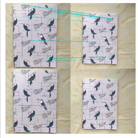
① 第一组数据
七点匹配点计算基础矩阵：
控制台输出：

461
461
36
[[  1.97239734e-07  -4.26561273e-05   2.52904527e-02]
 [  4.24989402e-05  -1.90178422e-06  -2.44330900e-02]
 [ -2.44701559e-02   2.30334778e-02   1.00000000e+00]]
1
2
3
4
5
6

结果图：

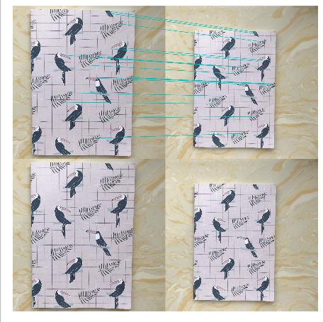
八点匹配点计算基础矩阵：
控制台输出：

461
461
29
[[ -2.55224960e-07  -3.00786795e-07   1.58976498e-03]
 [  2.89707522e-06   1.45441317e-07  -1.46080960e-02]
 [ -2.81378730e-03   1.23999326e-02   1.00000000e+00]]
1
2
3
4
5
6

结果图：

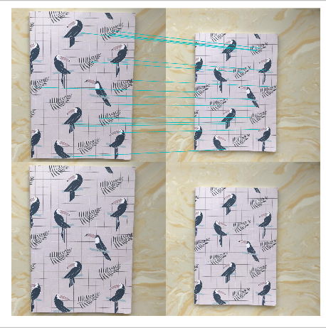
十点匹配点计算基础矩阵：
控制台输出：

processed tmp.pgm to im1.sift
processed tmp.pgm to im2.sift
461
461
36
[[  6.79062229e-06  -3.58141837e-06  -3.86536085e-02]
 [  4.48539039e-06  -1.53238078e-07  -5.44511839e-03]
 [  2.94374668e-02   3.04050052e-03   1.00000000e+00]]
1
2
3
4
5
6
7
8

结果图：

② 第二组数据
七点匹配点计算基础矩阵：
控制台输出：

734
734
32
[[  4.41348662e-08  -3.42650050e-06   2.34914137e-03]
 [  3.37627195e-06   3.86920082e-08  -2.77634118e-03]
 [ -2.51280140e-03   1.50309243e-03   1.00000000e+00]]
1
2
3
4
5
6

结果图：

八点匹配点计算基础矩阵：
控制台输出：

734
734
59
[[  5.13681399e-08  -2.72006999e-06   2.33030990e-03]
 [  2.71521610e-06   1.85826640e-08  -2.25616582e-03]
 [ -2.51198132e-03   1.22928879e-03   1.00000000e+00]]
1
2
3
4
5
6

结果图：

十点匹配点计算基础矩阵：
控制台输出：

734
734
46
[[  3.32345027e-08  -5.21542621e-06   1.99979624e-03]
 [  5.14872251e-06   2.89078827e-08  -6.53046230e-03]
 [ -2.23058142e-03   4.65965814e-03   1.00000000e+00]]
1
2
3
4
5
6

结果图：

③第三组数据
七点匹配点计算基础矩阵：
控制台输出：

632
632
28
[[  2.87480615e-06  -2.51191641e-04   1.83003566e-01]
 [  2.49457112e-04   3.69779415e-06  -1.27817047e-01]
 [ -1.69252496e-01   1.14233511e-01   1.00000000e+00]]
1
2
3
4
5
6

结果图：

八点匹配点计算基础矩阵：
控制台输出：

632
632
32
[[  3.78497574e-08   2.12332184e-05  -3.28211216e-02]
 [ -2.20359610e-05   4.36071279e-07   2.63780580e-02]
 [  3.62485855e-02  -2.94763915e-02   1.00000000e+00]]
1
2
3
4
5
6

结果图：

十点匹配点计算基础矩阵：
控制台输出：

632
632
53
[[  4.66996990e-08  -2.04474321e-05   1.99506699e-02]
 [  2.07208420e-05   2.14957900e-07  -1.06213988e-02]
 [ -2.00422549e-02   9.28538206e-03   1.00000000e+00]]
1
2
3
4
5
6

结果图：

实验分析：
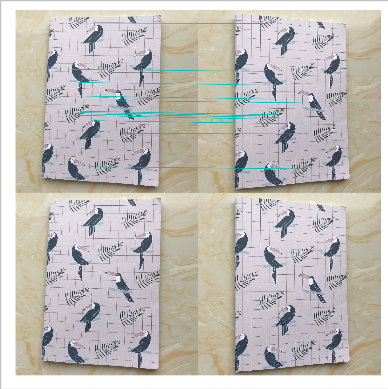
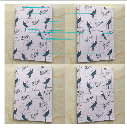
（1）由第一组的实验结果分析可得：随着改变参数7、8、10，即匹配点的个数，得到的基础矩阵是各不相同的，对基础矩阵的有非常大的影响；除此之外匹配点的个数对于最终得到的特征匹配图也有较大的影响，其规律不是特别明显，但当参数较大时，匹配线的数量较多。
（2）远近不同的图片组经过算法匹配效果相对于远近相同的图片组效果要差一些，甚至出现了明显的错误匹配，第一组的图片匹配点较多，但是优化后所剩下的较少，第二张匹配点相对第一组较少，但是优化过后明显特征的匹配点仍被保留。
（3）sift算法本身有时候会因为匹配点附近太过相似而出现错误匹配，这个算法便能在这个基础上相对优化，避开错误的匹配，但是以上的结果都出现了一个情况，优化后的结果仍存在错误的匹配点，整体效果并不好，由于图像远近以及光线的影响，呈现的效果也不够理想，而相对的，远近相同的测试图片效果会比远近相差较大的图片要好，更容易匹配。
（4）在本次实验中，三组数据相较来说，平移变换图像相比较其他两种构图方式的图像有着较多的特征匹配数，因为平移变换对物体特征点的影响较小，而远近和左右角度变换都会在不同程度上影响到特征点的收集和遮蔽。

3.3 极点与极线

3.3.1 实验代码

import numpy as np
import cv2 as cv
from matplotlib import pyplot as plt
def drawlines(img1, img2, lines, pts1, pts2):
    ''' img1 - image on which we draw the epilines for the points in img2
        lines - corresponding epilines '''
    r, c = img1.shape
    img1 = cv.cvtColor(img1, cv.COLOR_GRAY2BGR)
    img2 = cv.cvtColor(img2, cv.COLOR_GRAY2BGR)
    for r, pt1, pt2 in zip(lines, pts1, pts2):
        color = tuple(np.random.randint(0, 255, 3).tolist())
        x0, y0 = map(int, [0, -r[2] / r[1]])
        x1, y1 = map(int, [c, -(r[2] + r[0] * c) / r[1]])
        img1 = cv.line(img1, (x0, y0), (x1, y1), color, 1)
        img1 = cv.circle(img1, tuple(pt1), 5, color, -1)
        img2 = cv.circle(img2, tuple(pt2), 5, color, -1)
    return img1, img2
img1 = cv.imread('data/1.jpg', 0)  # queryimage # left image
img2 = cv.imread('data/2.jpg', 0)  # trainimage # right image
sift = cv.xfeatures2d.SIFT_create()
# find the keypoints and descriptors with SIFT
kp1, des1 = sift.detectAndCompute(img1, None)
kp2, des2 = sift.detectAndCompute(img2, None)
# FLANN parameters
FLANN_INDEX_KDTREE = 1
index_params = dict(algorithm=FLANN_INDEX_KDTREE, trees=5)
search_params = dict(checks=50)
flann = cv.FlannBasedMatcher(index_params, search_params)
matches = flann.knnMatch(des1, des2, k=2)
good = []
pts1 = []
pts2 = []
# ratio test as per Lowe's paper
for i, (m, n) in enumerate(matches):
    if m.distance < 0.8 * n.distance:
        good.append(m)
        pts2.append(kp2[m.trainIdx].pt)
        pts1.append(kp1[m.queryIdx].pt)
pts1 = np.int32(pts1)
pts2 = np.int32(pts2)
F, mask = cv.findFundamentalMat(pts1, pts2, cv.FM_LMEDS)
# We select only inlier points
pts1 = pts1[mask.ravel() == 1]
pts2 = pts2[mask.ravel() == 1]
# Find epilines corresponding to points in right image (second image) and
# drawing its lines on left image
lines1 = cv.computeCorrespondEpilines(pts2.reshape(-1, 1, 2), 2, F)
lines1 = lines1.reshape(-1, 3)
img5, img6 = drawlines(img1, img2, lines1, pts1, pts2)
# Find epilines corresponding to points in left image (first image) and
# drawing its lines on right image
lines2 = cv.computeCorrespondEpilines(pts1.reshape(-1, 1, 2), 1, F)
lines2 = lines2.reshape(-1, 3)
img3, img4 = drawlines(img2, img1, lines2, pts2, pts1)
plt.subplot(121), plt.imshow(img5)
plt.subplot(122), plt.imshow(img3)
plt.show()
1
2
3
4
5
6
7
8
9
10
11
12
13
14
15
16
17
18
19
20
21
22
23
24
25
26
27
28
29
30
31
32
33
34
35
36
37
38
39
40
41
42
43
44
45
46
47
48
49
50
51
52
53
54
55
56
57

3.3.2 实验结果及分析

① 第一组数据

② 第二组数据

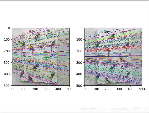
③ 第三组数据

实验分析：

对于第三组实验数据来说，极点为途中所有直线的交点处，由于改组图像为前后远近不同的图像组，所以该图像组的极线呈散射状，极点位于所有极线的交点处。

4. 实验中遇到的问题

在本次实验中遇到如下问题，在代码运行过程中遇到如下报错：

ImportError: cannot import name 'ransac'
1

解决方法：
将代码中的from PCV.geometry import ransac改为from PCV.tools import ransac即可，因为ransac.py文件夹在PCV下的tools文件夹内，不在geometry 内。