不正经

这个屌丝很懒，什么也没留下！

热门标签

连接时序分类 Connectionist Temporal Classiﬁcation (CTC)

作者：不正经 | 2024-03-15 06:02:02

踩

CTC全称Connectionist temporal classification，是一种常用在语音识别、文本识别等领域的算法，用来解决输入和输出序列长度不一、无法对齐的问题。在CRNN中，它实际上就是模型对应的损失函数(CTC loss)。

一、背景

字母和语音的对齐(align)非常困难而且容易出错的，因为很多音素的边界是很难区分。CTC不要求训练数据的对齐，因此非常适合语音识别和手写文字识别这种问题。

我们引入一些记号更加形式化的描述CTC要解决的问题。首先我们假设输入序列 $X = [x_1, x_2,..., x_T]$ ，比如在语音识别中，它是T个帧，每一帧 $x_t$ 是39维的MFCC特征。输出序列是 $Y=[y_1, y_2, ..., y_U]$ 。这个任务我们很难把它转化为简单的分类任务，因为：

X和Y都是变长的
X和Y的长度比也是变化的(X和Y的长度不存在简单的比例对应关系)
训练数据中没有X和Y的对齐

NLP的任务存在清晰的边界。NLP的输入和输出都是逻辑上的符号，每个符号的边界是显然的，但是语音信号的边界是模糊不清的。CTC可以解决这些问题，给定一个输入X，CTC可以对所有可能的Y计算 $P(Y \vert X)$ 。有了这个概率，我们就可以推断最可能的输出或者计算某个Y的概率。训练的时候，我们需要计算损失函数去更新参数。预测时，找到最可能的Y， $Y^*=\underset{Y}{argmax}P(Y|X)$ 。CTC虽然没有精确的算法来高效的计算最优路径，但是它提供近似的算法使得我们能在合理的时间内找到较优的路径。

二、CTC算法

给定X时，CTC算法可以计算所有输出Y的概率。去计算我们需要解决1. 对齐 2. 损失函数

1. 对齐

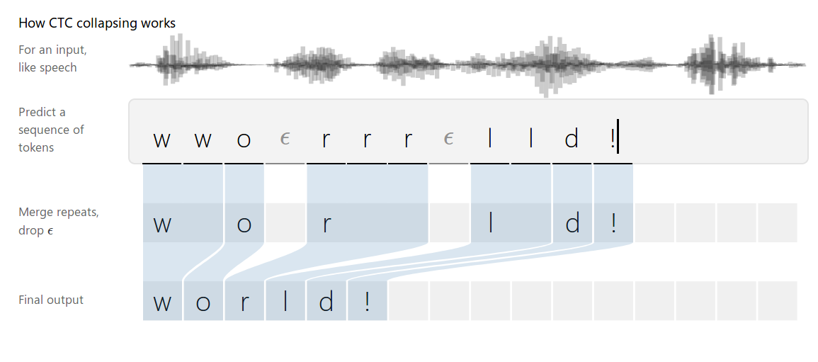
CTC算法不需要对齐输入和输出的。CTC会枚举所有可能的对齐方式然后把这些概率累积起来。先来尝试一个简单的对齐，每个输入对应一个字符：

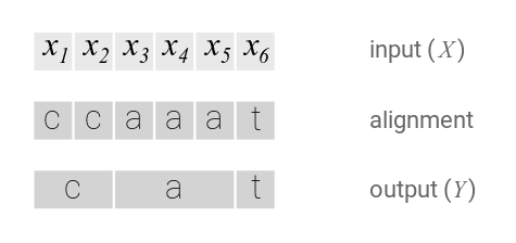
这种简单的对齐有两个问题：

每个输入不一定都对应实际的输出。
比如在语音识别中会有静音(silence)，这些输入不对应任何输出
没办法输出连续相同的字符。
比如假设有一个单词caat，那么上面的对齐只能认为输出是cat。

为了解决上述问题，CTC引入了一个新的特殊符号 $\epsilon$ ，它表示空字符，在最后我们会去掉它。

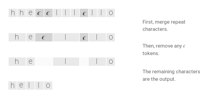
如果输出有两个连续相同的字符，那么它们之间一定要有至少一个空字符，这样我们就可以区分hello和helo了。CTC对齐有如下一些特性。首先对齐是单调的（monotonic），If we advance to the next input, we can keep the corresponding output the same or advance to the next one.。第二个特点就是输入与输出是多对一的关系。这个特性可以推出如下结论：输入序列的长度一定是大于等于输出长度的。

2. 损失函数

The CTC alignments give us a natural way to go from probabilities at each time-step to the probability of an output sequence.

上图中，RNN模型会计算每一个时刻t的输出的概率分布 $p_t(a \vert X)$ ，表示t时刻输出字符a的概率。假设输入的长度为T，那么理论上有5^T中不同的对齐方式（路径），当然有些概率很低，我们可以忽略。这些路径中有一些的输出是一样的，比如都是”hello”，我们把它的概率加起来就得到了 $P("hello" \vert X)$ 的概率。即：

$P(Y|X)= \underset{A \in \mathcal{A}_{X,Y}}{\sum} \prod_{t=1}^{T}p_t(a_t|X)$ (marginalizes over the set of valid alignments)

给定X和Y，如果我们直接遍历所有的路径，那么效率会非常低，因为路径会随着T指数增加。不过我们可以使用动态规划技术来提高计算效率。Thankfully, we can compute the loss much faster with a dynamic programming algorithm. The key insight is that if two alignments have reached the same output at the same step, then we can merge them.

Since we can have an ϵ before or after any token in Y, it’s easier to describe the algorithm using a sequence which includes them. We’ll work with the sequence

$Z=[\epsilon, y_1, \epsilon, y_2, ..., y_U, \epsilon]$

which is Y with an ϵ at the beginning, end, and between every character.

let $\alpha$ be the score of the merged alignments at a given node. More precisely, $\alpha_{s,t}$ is the CTC score of the subsequence $Z_{1:s}$ after $t$ input steps. As we’ll see, we’ll compute the final CTC score, $P(Y|X)$ , from the $\alpha$ ’s at the last time-step. As long as we know the values of $\alpha$ at the previous time-step, we can compute $\alpha_{s,t}$ . There are two cases.

Case 1: 不能跳过 z_{s-1}。
原因：z_{s-1}可能是Y中的元素，即z_s = ϵ
**z_{s-1}是**ϵ **来分割相同的两个元素，即z_s = z_{s-2}**

**Case 2: 能跳过 z_{s-1}。**
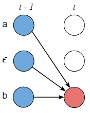
当 **z_{s-1}是两个独特的元素之间的**ϵ

具体的：

Case 1： $\alpha_{s,t} = (\alpha_{s-1,t-1}+\alpha_{s,t-1}) \cdot p_t(z_s|X)$
Case 2： $\alpha_{s,t} = (\alpha_{s-2,t-1} + \alpha_{s-1,t-1}+\alpha_{s,t-1}) \cdot p_t(z_s|X)$

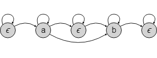
Below is an example of the computation performed by the dynamic programming algorithm. Every valid alignment has a path in this graph.

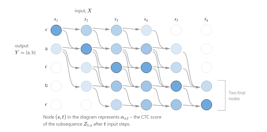
There are two valid starting nodes and two valid final nodes since the ϵ at the beginning and end of the sequence is optional. The complete probability is the sum of the two final nodes.

Now that we can efficiently compute the loss function, the next step is to compute a gradient and train the model. The CTC loss function is differentiable with respect to the per time-step output probabilities since it’s just sums and products of them. Given this, we can analytically compute the gradient of the loss function with respect to the (unnormalized) output probabilities and from there run backpropagation as usual.

For a training set $\mathcal{D}$ , the model’s parameters are tuned to minimize the negative log-likelihood

$L=\underset{(X,Y) \in \mathcal{D}}{\sum}-log P(Y|X)$

instead of maximizing the likelihood directly.

3. 预测 Inference

模型训练好了之后，我们需要用它来预测最可能的结果。具体来说，我们需要解决如下问题：

$Y^*=\underset{Y}{argmax}P(Y|X)$

可以用贪心算法，每个时间步都取概率最大的对齐。但其没有考虑到单个输出可能有多种对齐。举个例子，Assume the alignments [a, a, ϵ] and [a, a, a] individually have lower probability than [b, b, b]. But the sum of their probabilities is actually greater than that of [b, b, b]. The naive heuristic will incorrectly propose Y= [b] as the most likely hypothesis. It should have chosen Y= [a].

我们可以使用一个改进版的Beam Search方法来搜索，虽然它不能保证找到最优解，但是我们可以调整beam的大小，beam越小，速度越快；beam越大，搜索的解越好。极限的情况是，如果beam是1那么它等价与前面的算法；如果beam是所有字母的个数，那么它会遍历所有路径，保证能找到最优解。

普通的Beam Search方法会在每个时刻保留最优的N条路径，然后在t+1时刻对这N条路径展开，然后从所有展开的路径中选择最优的N条路径，一直到最终时刻T。下图是使用普通Beam Search算法的示例（beam大小=3）。在图中，我们发现在t=3的时候，有两条路径的输出都是a(分别是[a,ϵ]和[ϵ,a]），它们(有可能)是可以合并的。

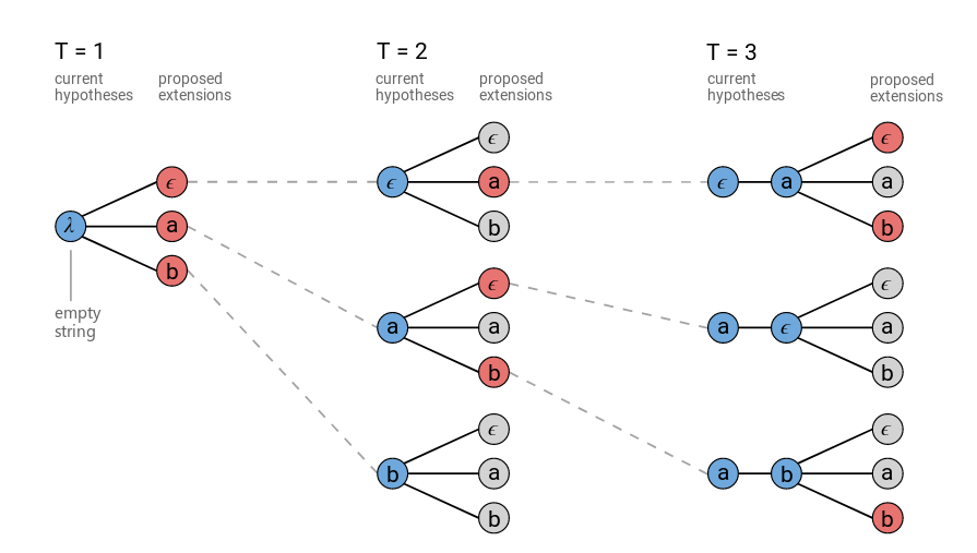
因此我们可以改进一些Beam Search算法，把相同输出的路径合并起来。这里的合并是把输出里相同的字符变成一个，并且去掉空字符，然后所有相同输出的概率累加起来。

改进后的算法的搜索过程如下图（beam大小为3）。

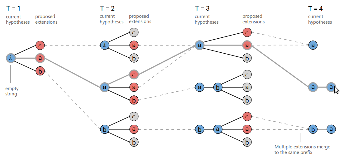
在t=3的时刻，在下方，[b,a,ϵ] 和 [b,a,a] 被合并成相同的结果[b,a]。另外需要注意的是t=3的时刻，上方[a]在扩展增加a的时候会输出两条路径：[a,a]与[a]。

A proposed extension can map to two output prefixes if the character is a repeat. This is shown at T=3 in the figure above where ‘a’ is proposed as an extension to the prefix [a]. Both [a] and [a, a] are valid outputs for this proposed extension.

When we extend [a] to produce [a,a], we only want include the part of the previous score for alignments which end in ϵ. Remember, the ϵ is required between repeat characters. Similarly, when we don’t extend the prefix and produce [a], we should only include the part of the previous score for alignments which don’t end in ϵ.

Given this, we have to keep track of two probabilities for each prefix in the beam. The probability of all alignments which end in ϵ and the probability of all alignments which don’t end in ϵ. When we rank the hypotheses at each step before pruning the beam, we’ll use their combined scores.

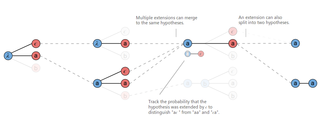
The implementation of this algorithm doesn’t require much code, but it is dense and tricky to get right. Checkout this gist for an example implementation in Python.

In some problems, such as speech recognition, incorporating a language model over the outputs significantly improves accuracy. We can include the language model as a factor in the inference problem.

The function $L(Y)$ computes the length of $Y$ in terms of the language model tokens and acts as a word insertion bonus. With a word-based language model $L(Y)$ counts the number of words in $Y$ . If we use a character-based language model then $L(Y)$ counts the number of characters in $Y$ . The language model scores are only included when a prefix is extended by a character (or word) and not at every step of the algorithm. This causes the search to favor shorter prefixes, as measured by $L(Y)$ , since they don’t include as many language model updates. The word insertion bonus helps with this. The parameters $\alpha$ and $\beta$ are usually set by cross-validation.

The language model scores and word insertion term can be included in the beam search. Whenever we propose to extend a prefix by a character, we can include the language model score for the new character given the prefix so far.

三、CTC算法的性质

We mentioned a few important properties of CTC so far. Here we’ll go into more depth on what these properties are and what trade-offs they offer.

1. Conditional Independence 条件独立

CTC的一个缺点是它的条件独立假设。The model assumes that every output is conditionally independent of the other outputs given the input. This is a bad assumption for many sequence to sequence problems.

Say we had an audio clip of someone saying “triple A”. Another valid transcription could be “AAA”. If the first letter of the predicted transcription is ‘A’, then the next letter should be ‘A’ with high probability and ‘r’ with low probability. The conditional independence assumption does not allow for this.

If we predict an ‘A’ as the first letter then the suffix ‘AA’ should get much more probability than ‘riple A’. If we predict ‘t’ first, the opposite should be true.

In fact speech recognizers using CTC don’t learn a language model over the output nearly as well as models which are conditionally dependent. However, a separate language model can be included and usually gives a good boost to accuracy.

The conditional independence assumption made by CTC isn’t always a bad thing. Baking in strong beliefs over output interactions makes the model less adaptable to new or altered domains. For example, we might want to use a speech recognizer trained on phone conversations between friends to transcribe customer support calls. The language in the two domains can be quite different even if the acoustic model is similar. With a CTC acoustic model, we can easily swap in a new language model as we change domains.

2. Alignment Properties

CTC算法不需要训练数据对齐，它会把所有相同输出的对齐合并。虽然CTC要求输入X和输出Y严格对齐，但是具体怎么对齐它并没有在模型层面加任何限制，是把概率比较均匀的分配给所有可能的路径还是把概率集中的分配给某些路径，这是不能确定的。

CTC要求对齐的方式是单调的monotonic alignments，这对于语音识别是合适的假设，但是对于其它的任务，比如机器翻译，这种对齐是不合适的。因为一个不同语言的语序是不同的，比如英语a friend of mine和我的朋友，在英语里，friend在mine之前，但是在汉语里”我的”在”朋友”之前。

CTC的另外一个要求就是输入和输出是多对一的，有的任务可以要求严格的一对一关系，比如词性标注，那CTC也是不合适的。另外它也无法表示输入与输出的多对一的关系。比如在英语中，th是一个音素，一个输入可能要对于th这两个输出，CTC也是无法表示这种关系的。

最后一个就是CTC隐式说明输出一定比输入短，虽然这在语音识别是合理的假设（因为输入都很长），但是其它的任务可能就不一定。

四、CTC与序列模型关系 CTC in Context

In this section we’ll discuss how CTC relates to other commonly used algorithms for sequence modeling.

1. HMMs

Hidden Markov Model (HMM) and CTC are actually quite similar. Understanding the relationship between them will help us understand what advantages CTC has over HMM sequence models and give us insight into how CTC could be changed for various use cases.

**CTC HMM:** The first two nodes are the starting states and the last two nodes are the final states.

References

单篇

CTC理论和实战 - 李理的博客

Sequence Modeling with CTC

Listen, Attend and Spell: A Neural Network for Large Vocabulary Conversational Speech Recognition [PDF]
Chan, W., Jaitly, N., Le, Q.V. and Vinyals, O., 2016. ICASSP.
Exploring Neural Transducers for End-to-End Speech Recognition [PDF]
Battenberg, E., Chen, J., Child, R., Coates, A., Gaur, Y., Li, Y., Liu, H., Satheesh, S., Seetapun, D., Sriram, A. and Zhu, Z., 2017.
Connectionist Temporal Classification : Labelling Unsegmented Sequence Data with Recurrent Neural Networks [PDF]
Graves, A., Fernandez, S., Gomez, F. and Schmidhuber, J., 2006. Proceedings of the 23rd international conference on Machine Learning, pp. 369--376. DOI: 10.1145/1143844.1143891

汇总：

深度学习理论与实战：提高篇 - 李理的博客

声明：本文内容由网友自发贡献，不代表【wpsshop博客】立场，版权归原作者所有，本站不承担相应法律责任。如您发现有侵权的内容，请联系我们。转载请注明出处：https://www.wpsshop.cn/w/不正经/article/detail/239192