
- 1valser网站(计算机视觉CV,CG学习交流社区)_valser.org
- 2编程式导航router.push(...)中传参的两种方式query和params及两者区别_router.push params query
- 3Spring Boot+JSP启动报404错误找不到页面_jsp项目部署不能找到登陆界面
- 4实现图像检索系统需要用到哪方面的知识?
- 5华为HCIP-DATACOM题库解析71-110(821)_当两端bfd检测时间间隔分别为30ms
- 6springboot+vue房产中介管理信息系统
- 7java camel命名_Java篇—驼峰命名法(CamelCase)
- 8mac或者linux下安装composer phalcon debug
- 9快速排序算法 C语言实现_c语言完整的快速排序算法
- 10第十八届全国大学生智能车竞赛签到信息_苏州城市学院李想
复杂网络与NetworkX——有向图与无向图的绘制
赞
踩

目录
一、networkx介绍
NetworkX是一个用于创建、操作和研究复杂网络的Python库。它提供了广泛的功能,使用户能够生成各种类型的图形、执行常见的图形操作、分析图形的属性以及可视化网络结构。
以下是一些NetworkX的主要特点和功能:
-
创建和操作图形:NetworkX允许用户创建多种类型的图形,包括无向图、有向图、加权图等。它提供了简单的接口来添加节点和边,并支持常见的图形操作,如添加、删除和修改节点和边。
-
图形分析和算法:NetworkX提供了许多图形分析和算法工具,使用户能够研究和分析网络的各种属性和特征。例如,可以计算图形的度分布、最短路径、连通性、聚类系数、中心性指标等。
-
图形生成器:NetworkX提供了多种图形生成器,用于生成具有特定特征的图形。例如,可以使用随机图生成器生成随机网络、使用小世界图生成器生成小世界网络,或使用Barabasi-Albert图生成器生成无标度网络。
-
可视化:NetworkX支持将图形可视化,以便更直观地理解和呈现网络结构。它可以使用各种布局算法将节点和边进行可视化,并提供灵活的参数控制来调整可视化效果。
-
扩展性:NetworkX具有高度的可扩展性,可以与其他Python科学计算库(如NumPy、SciPy和Pandas)进行集成。这使得用户能够利用其他库的功能来扩展NetworkX的功能。
二、复杂网络介绍
复杂网络是由大量节点和它们之间的连接所组成的网络结构,其中节点和连接之间存在着非常丰富和复杂的关系。与简单网络(如正则网络或完全图)相比,复杂网络更贴近现实世界的各种真实系统,如社交网络、互联网、神经网络、物流网络等。
复杂网络的特点和性质包括:小世界性质、无标度性质、社区结构、高鲁棒性;
钱学森给出了复杂网络的一个较严格的定义:具有自组织、自相似、吸引子、小世界、无标度中部分或全部性质的网络称为复杂网络。
-
自组织性(Self-organization):指复杂网络在没有外部控制或指导的情况下,能够通过节点之间的相互作用和调整,形成一种自发的组织结构。这种自组织性使得网络能够在动态环境中适应和演化。
-
自相似性(Self-similarity):表示复杂网络在不同的尺度上具有类似的结构和特征。换句话说,网络的一部分与整体具有相似的性质,这种特性在多个层次上都存在。
-
吸引子(Attractor):指复杂网络在演化过程中的稳定状态或动态行为,可以被看作是网络的吸引子。吸引子可以是节点或节点集合,具有稳定性和吸引其他节点的特性。
-
小世界性(Small-world):指复杂网络中的节点之间平均最短路径长度较短,且聚集性较高。这意味着网络中任意两个节点之间通过少数的中间节点即可相互连通,同时节点之间呈现出一定的聚类或簇状结构。
-
无标度性(Scale-free):表示复杂网络的度分布呈现幂律分布,即只有少数几个节点具有非常高的度数,而大多数节点的度数相对较低。这种无标度性质意味着网络中存在少数核心节点,它们对整个网络的结构和功能具有重要影响。
三、图的介绍
Graph(图)是由一组节点(vertices)和连接它们的边(edges)组成的数据结构。它用于表示实体之间的关系或相互作用,并提供了一种可视化和分析这些关系的方式。图是图论的基础,广泛应用于计算机科学、社会网络分析、物流规划、生物网络等领域。
下面是一些图的基本概念和特性:
-
节点(Vertices):也称为顶点或节点,表示图中的实体或元素。节点可以表示个人、物体、事件等。
-
边(Edges):也称为连接、关系或弧,表示节点之间的关联关系。边可以是有向的(从一个节点指向另一个节点)或无向的(没有方向性)。
-
权重(Weights):可选属性,用于表示边的强度、距离或其他度量。
-
路径(Path):是指图中的一系列边,沿着这些边可以从一个节点到达另一个节点。
-
度(Degree):节点的度是指与该节点相连的边的数量。对于有向图,分为入度(In-degree)和出度(Out-degree)。
根据图的性质和结构,可以将图分为不同的类型,包括但不限于以下几种:
-
无向图(Undirected Graph):图中的边没有方向性,即可以沿着边双向移动。例如,社交网络中的好友关系图可以被建模为无向图。
-
有向图(Directed Graph):图中的边具有方向性,即从一个节点指向另一个节点。例如,互联网中的网页链接关系可以被建模为有向图。
-
加权图(Weighted Graph):图中的边带有权重,用于表示边的强度、距离或其他度量。例如,交通网络中的道路可以被建模为加权图,权重可以表示道路的长度或拥堵程度。
-
多重图(Multigraph):图中的边允许重复,即可以存在多个相同的边连接同一对节点。例如,通信网络中的多条通信线路可以被建模为多重图。
-
带环图(Cyclic Graph)和无环图(Acyclic Graph):带环图包含至少一个环(环是指从一个节点出发,经过一系列边回到原始节点的路径),而无环图不包含任何环。
那我们应该如何根据实际情况选择使用哪种图呢?
-
无向图 vs. 有向图:
- 如果问题中的关系是无方向性的,或者您只关注节点之间的连接而不考虑方向,那么无向图是一个合适的选择。
- 如果问题中的关系具有明确的方向性,并且节点之间的连接有向而非双向,那么有向图是更合适的选择。
-
加权图 vs. 非加权图:
- 如果问题中的边具有权重或强度的概念,并且您需要考虑边的权重作为网络结构和分析的一部分,那么加权图是适合的选择。
- 如果问题中的边没有权重或者权重对问题的解决没有实质性影响,那么非加权图可以满足需求。
-
多重图 vs. 单重图:
- 如果问题中的节点之间允许多个相同类型的边存在,并且您需要考虑并分析这些多个边的信息,那么多重图是一个合适的选择。
- 如果问题中的节点之间只存在单个连接关系,并且不需要考虑重复的边,那么单重图可以满足需求。
-
带环图 vs. 无环图:
- 如果问题中的节点之间存在环(环是指从一个节点出发,经过一系列边回到原始节点的路径),并且您需要考虑环的影响和分析环的特性,那么带环图是一个合适的选择。
- 如果问题中的节点之间不存在环,或者环对问题的解决没有实质性影响,那么无环图可以满足需求。
下面为创建几个图的方式:
- 创建无向图(Undirected Graph):
- import networkx as nx
- # 创建一个空的无向图
- G = nx.Graph()
- # 添加节点
- G.add_nodes_from([1, 2, 3, 4])
- # 添加边
- G.add_edges_from([(1, 2), (2, 3), (3, 4), (4, 1)])
- # 或者可以使用下面的方式一次性添加边
- # edges = [(1, 2), (2, 3), (3, 4), (4, 1)]
- # G.add_edges_from(edges)
- 创建有向图(Directed Graph):
- import networkx as nx
- # 创建一个空的有向图
- G = nx.DiGraph()
- # 添加节点
- G.add_nodes_from([1, 2, 3, 4])
- # 添加有向边
- G.add_edges_from([(1, 2), (2, 3), (3, 4), (4, 1)])
- # 或者可以使用下面的方式一次性添加有向边
- # edges = [(1, 2), (2, 3), (3, 4), (4, 1)]
- # G.add_edges_from(edges)
- 创建加权图(Weighted Graph):
- import networkx as nx
- # 创建一个空的加权图
- G = nx.Graph()
- # 添加节点
- G.add_nodes_from([1, 2, 3, 4])
- # 添加带权边
- G.add_weighted_edges_from([(1, 2, 0.5), (2, 3, 1.2), (3, 4, 0.8), (4, 1, 1.5)])
- # 或者可以使用下面的方式一次性添加带权边
- # weighted_edges = [(1, 2, 0.5), (2, 3, 1.2), (3, 4, 0.8), (4, 1, 1.5)]
- # G.add_weighted_edges_from(weighted_edges)
- 创建多重图(Multigraph):
- import networkx as nx
- # 创建一个空的多重图
- # G = nx.MultiGraph() # 创建多重无向图
- # G = nx.MultiDigraph() # 创建多重有向图
- G = nx.MultiGraph()
- # 添加节点
- G.add_nodes_from([1, 2, 3, 4])
- # 添加多重边
- G.add_edges_from([(1, 2), (1, 2), (2, 3), (3, 4)])
- 创建带环图(Cyclic Graph):
- import networkx as nx
- # 创建一个带环的有向图
- G = nx.DiGraph()
- # 添加节点
- G.add_nodes_from([1, 2, 3, 4])
- # 添加有向边,形成环
- G.add_edges_from([(1, 2), (2, 3), (3, 4), (4, 1)])
G.clear() #清空图更多相关内容请看官网:教程 — NetworkX 3.1 文档
四、网络的统计指标
-
节点数(Number of nodes):表示网络中的节点数量,用来衡量网络规模的大小。
-
边数(Number of edges):表示网络中的边数量,用来描述节点之间的连接关系。
-
平均度(Average degree):计算网络中所有节点的度的平均值,度是指与节点相连的边的数量。平均度反映了网络的连接密度和复杂程度。
-
聚集系数(Clustering coefficient):用于衡量节点邻居之间的紧密程度。聚集系数可以用来评估网络中节点的集聚性和社区结构。
-
最短路径长度(Shortest path length):表示网络中任意两个节点之间最短路径的长度。最短路径长度用来衡量节点之间的距离和网络的“小世界”性质。
-
中心性(Centrality):衡量节点在网络中的重要性或影响力。常见的中心性指标包括度中心性(Degree centrality)、介数中心性(Betweenness centrality)和接近中心性(Closeness centrality)等。
-
度分布(Degree distribution):描述节点度数的概率分布。度分布可以用来研究网络的无标度性质和节点的重要性分布。
-
社区结构(Community structure):用于描述网络中的子图或社区,其中节点在同一社区内紧密连接,而社区之间的连接相对稀疏。
-
同配性(Assortativity):衡量节点倾向于与具有相似度的节点连接的程度。同配性可以用来研究网络中节点的偏好和社群结构。
-
强连通分量(Strongly connected components):对于有向图,强连通分量是指其中任意两个节点之间都存在有向路径的节点子集。
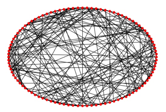
五、基础教程
- #添加节点
- import networkx as nx
- import matplotlib.pyplot as plt
- G = nx.Graph() #建立一个空的无向图G
- G.add_node('1') #添加一个节点1
- nx.draw(G, with_labels=True)
- plt.show()
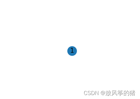
- G.add_nodes_from(['2','3','4','5']) #加点集合
- nx.draw(G, with_labels=True)
- plt.show()
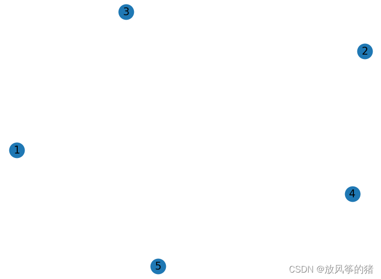
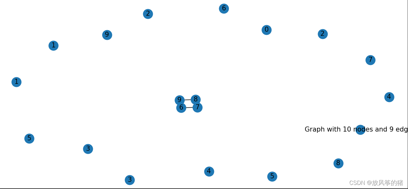
- G.add_cycle(['6', '7', '8', '9']) # 加环
- G.add_edges_from([('6', '7'), ('7', '8'), ('8', '9'), ('9', '6')]) # 添加边
- nx.draw(G, with_labels=True)
- plt.show()
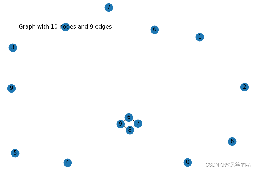
- H = nx.path_graph(10) #返回由10个节点挨个连接的无向图,所以有9条边
- G.add_nodes_from(H) #创建一个子图H加入G
- G.add_node(H) #直接将图作为节点
- nx.draw(G, with_labels=True)
- plt.show()
- #访问节点
- print('图中所有的节点', G.nodes())
- print('图中节点的个数', G.number_of_nodes())
图中所有的节点 ['1', '2', '3', '4', '5', '6', '7', '8', '9', 0, 1, 2, 3, 4, 5, 6, 7, 8, 9, <networkx.classes.graph.Graph object at 0x00000237BEC80A90>]
图中节点的个数 20
- G.remove_node(1) #删除指定节点
- G.remove_nodes_from(['2','3','4','5']) #删除集合中的节点
- nx.draw(G, with_labels=True)
- plt.show()
- #添加边
- F = nx.Graph() # 创建无向图
- F.add_edge(11,12) #一次添加一条边
- nx.draw(F, with_labels=True)
- plt.show()

- e=(13,14) #e是一个元组
- F.add_edge(*e) #这是python中解包裹的过程
- nx.draw(F, with_labels=True)
- plt.show()

- F.add_edges_from([(1,2),(1,3)])#通过添加list来添加多条边
- nx.draw(F, with_labels=True)
- plt.show()

- #通过添加任何ebunch来添加边
- F.add_edges_from(H.edges()) #不能写作F.add_edges_from(H)
- nx.draw(F, with_labels=True)
- plt.show()

- #访问边
- print('图中所有的边', F.edges())
- print('图中边的个数', F.number_of_edges())
图中所有的边 [(11, 12), (13, 14), (1, 2), (1, 3), (1, 0), (2, 3), (3, 4), (4, 5), (5, 6), (6, 7), (7, 8), (8, 9)]
图中边的个数 12
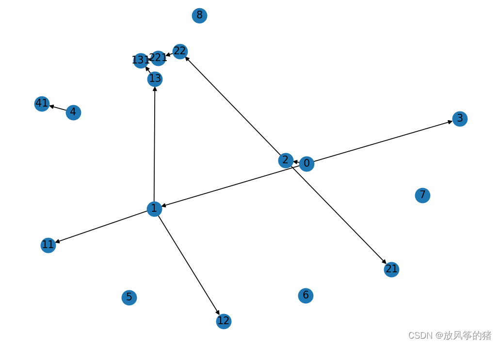
- #实例:在networkx中列出节点和边
- import networkx as nx
- import matplotlib.pyplot as plt
- G = nx.DiGraph()
- G.add_edges_from([('0', '1'), ('0', '2'), ('0', '3')])
- G.add_edges_from([('4', '41'), ('1', '11'), ('1', '12'), ('1', '13')])
- G.add_edges_from([('2', '21'), ('2', '22')])
- G.add_edges_from([('13', '131'), ('22', '221')])
- G.add_edges_from([('131', '221'), ('221', '131')])
- G.add_nodes_from(['5','6','7','8'])
- nx.draw(G, with_labels=True)
- plt.show()
六、手写数字无向图和有向图实例
无向图的构造:
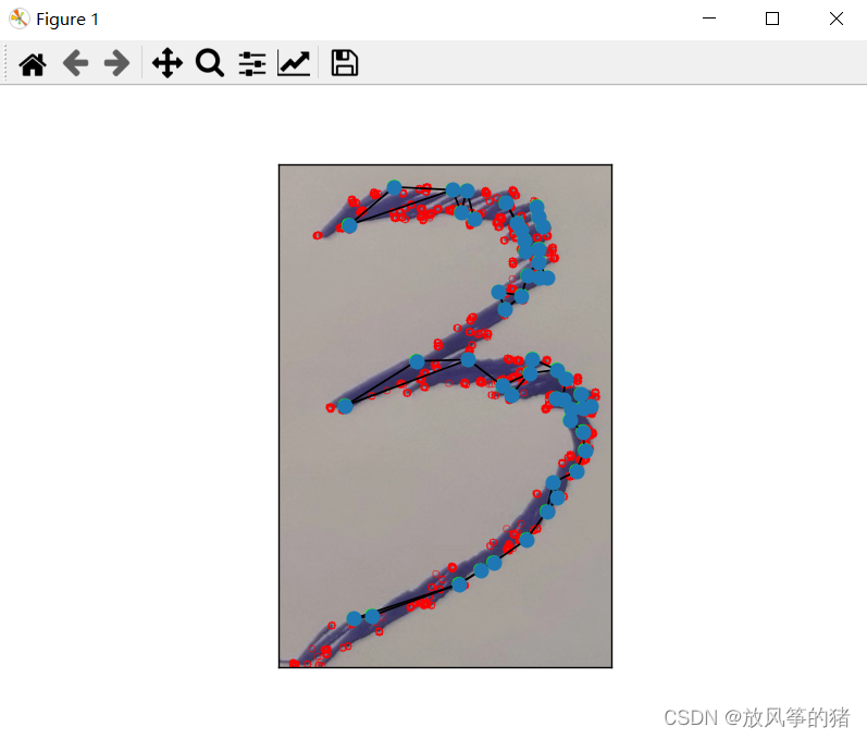
读取图像并进行灰度化处理:
使用OpenCV库读取图像,并将其转换为灰度图像。然后将图像转换为浮点型数据类型。
- image = cv2.imread("./num/0_4.jpg")
- gray_img = cv2.cvtColor(image, cv2.COLOR_BGR2GRAY)
- gray_img = np.float32(gray_img)
进行角点检测:
使用cv2.cornerHarris函数检测图像中的角点。
corners_img = cv2.cornerHarris(gray_img, block_size, sobel_size, k)
选择特征点:
使用cv2.goodFeaturesToTrack函数选择图像中的前num_keypoints个角点作为特征点。
- num_keypoints = 50
- corners = cv2.goodFeaturesToTrack(gray_img, num_keypoints, 0.01, 10)
- corners = np.intp(corners)
构建特征向量和图:
在这里,我们使用特征点的坐标构建了一个特征向量,并使用NetworkX库创建了一个无向图。图中的每个节点代表一个特征点,节点的位置属性(pos)表示特征点在图像上的位置。然后,根据最近邻原则,将每个节点与其两个最近的邻居节点连接起来。
- feature_vector = np.zeros((num_keypoints, 2))
-
- for i, corner in enumerate(corners):
- x, y = corner.ravel()
- feature_vector[i] = [x, y]
- G.add_node(i, pos=(x, y))
-
- for i in range(len(feature_vector)):
- distances = np.sqrt(np.sum((feature_vector - feature_vector[i])**2, axis=1))
- closest_neighbors = np.argsort(distances)[1:3]
- for neighbor in closest_neighbors:
- G.add_edge(i, neighbor, weight=1)
完整代码:
- import cv2
- import networkx as nx
- import numpy as np
- from matplotlib import pyplot as plt
-
- # detector parameters
- block_size = 3
- sobel_size = 3
- k = 0.06
-
- image = cv2.imread("./num/0_4.jpg")
- gray_img = cv2.cvtColor(image, cv2.COLOR_BGR2GRAY)
- gray_img = np.float32(gray_img)
-
- # detect the corners with appropriate values as input parameters
- corners_img = cv2.cornerHarris(gray_img, block_size, sobel_size, k)
-
- # set the number of keypoints to be selected
- num_keypoints = 50
-
- # find the top num_keypoints corners in the corners_img
- corners = cv2.goodFeaturesToTrack(gray_img, num_keypoints, 0.01, 10)
- corners = np.intp(corners)
-
- # create an empty feature vector with n dimensions
- feature_vector = np.zeros((num_keypoints, 2))
-
- # iterate over the corners and construct the feature vector
- for i, corner in enumerate(corners):
- x, y = corner.ravel()
- feature_vector[i] = [x, y]
- # print the extracted keypoints
- print("Keypoint %d: x=%d, y=%d" % (i+1, x, y))
-
- # create an empty graph
- G = nx.Graph()
-
- # add nodes to the graph
- for i, feature in enumerate(feature_vector):
- x, y = feature
- G.add_node(i, pos=(x, y))
-
- # add edges to the graph (connecting each node to its two closest neighbors)
- for i in range(len(feature_vector)):
- distances = np.sqrt(np.sum((feature_vector - feature_vector[i])**2, axis=1))
- closest_neighbors = np.argsort(distances)[1:3] # exclude the node itself
- for neighbor in closest_neighbors:
- G.add_edge(i, neighbor, weight=1)
-
- # draw the graph
- pos = nx.get_node_attributes(G, 'pos')
- nx.draw_networkx(G, pos=pos, with_labels=False, node_size=50)
-
- # show the image with the detected corners and feature vector
- for r in range(image.shape[0]):
- for c in range(image.shape[1]):
- pix = corners_img[r, c]
- if pix > 0.05 * corners_img.max():
- cv2.circle(image, (c, r), 5, (0, 0, 255), 0)
-
- # plot the feature vector on the image
- for i in range(num_keypoints):
- x, y = feature_vector[i]
- cv2.circle(image, (int(x), int(y)), 10, (0, 255, 0), -1)
-
- # convert the image back to RGB format
- image = cv2.cvtColor(image, cv2.COLOR_BGR2RGB)
-
- # display the image
- plt.imshow(image)
- plt.show()
有向图的构造:

完整代码:
- import cv2
- import networkx as nx
- import numpy as np
- from matplotlib import pyplot as plt
-
- # detector parameters
- block_size = 3
- sobel_size = 3
- k = 0.06
-
- image = cv2.imread("./num/0_7.jpg")
- gray_img = cv2.cvtColor(image, cv2.COLOR_BGR2GRAY)
- gray_img = np.float32(gray_img)
-
- # detect the corners with appropriate values as input parameters
- corners_img = cv2.cornerHarris(gray_img, block_size, sobel_size, k)
-
- # set the number of keypoints to be selected
- num_keypoints = 50
-
- # find the top num_keypoints corners in the corners_img
- corners = cv2.goodFeaturesToTrack(gray_img, num_keypoints, 0.01, 10)
- corners = np.intp(corners)
-
- # create an empty feature vector with n dimensions
- feature_vector = np.zeros((num_keypoints, 2))
-
- # iterate over the corners and construct the feature vector
- for i, corner in enumerate(corners):
- x, y = corner.ravel()
- feature_vector[i] = [x, y]
-
- # create an empty directed graph
- G = nx.DiGraph()
-
- # add nodes to the graph
- for i, feature in enumerate(feature_vector):
- x, y = feature
- G.add_node(i, pos=(x, y))
-
- # add edges to the graph
- for i in range(len(feature_vector)):
- distances = np.sqrt(np.sum((feature_vector[i] - feature_vector)**2, axis=1))
- closest_indices = np.argsort(distances)[1:3]
- for j in closest_indices:
- G.add_edge(i, j, weight=1)
-
- # draw the graph
- pos = nx.get_node_attributes(G, 'pos')
- nx.draw_networkx(G, pos=pos, with_labels=False, node_size=50)
-
- # show the image with the detected corners and feature vector
- for r in range(image.shape[0]):
- for c in range(image.shape[1]):
- pix = corners_img[r, c]
- if pix > 0.05 * corners_img.max():
- cv2.circle(image, (c, r), 5, (0, 0, 255), 0)
-
- # plot the feature vector on the image
- for i in range(num_keypoints):
- x, y = feature_vector[i]
- cv2.circle(image, (int(x), int(y)), 10, (0, 255, 0), -1)
-
- # convert the image back to RGB format
- image = cv2.cvtColor(image, cv2.COLOR_BGR2RGB)
-
- # display the image
- plt.imshow(image)
- plt.show()
参考链接:

