
- 1docker之基础命令相关操作上_usage: docker exec [options] container command [ar
- 2数字图像处理学习笔记4:图像增强之空间滤波2(一阶微分锐化滤波(梯度),二阶微分锐化(拉普拉斯),非锐化掩蔽)_拉普拉斯二阶微分锐化
- 3Eclipse连接SQL Server,JDBC Driver_eclipse连接sql怎么选jdbc驱动
- 4机器学习系列——(十一)回归
- 5第一章 ESP8266开发环境的搭建以及点亮板载小灯
- 6unity怎么设置分辨率_unity游戏分辨率怎么调
- 7JAVA 时间戳转化成时间的三种写法_timestamp数字转为时间
- 8漫谈重参数:从正态分布到Gumbel Softmax_正态分布重参数化
- 9Pytorch 如何高效使用GPU_torch划分gpu资源
- 10Java从HashSet中取元素_java hash set取值
【神经网络】(5) 卷积神经网络(ResNet50),案例:艺术画作10分类,附数据集_使用resnet50实现10种植物分类使用迁移学习构建网络
赞
踩
各位同学好,今天和大家分享一下TensorFlow2.0中如何构建卷积神经网络ResNet-50,案例内容:现在收集了10位艺术大师的画作,采用卷积神经网络判断某一幅画是哪位大师画的。
数据集:百度网盘 请输入提取码
提取码: 2h5x
1. 数据加载
在文件夹中将图片按照训练集、验证集、测试集划分好之后,使用tf.keras.preprocessing.image_dataset_from_directory()从文件夹中读取数据。指定参数label_model,'int'代表目标值y是数值类型,即0, 1, 2, 3等;'categorical'代表onehot类型,对应索引的值为1,如图像属于第二类则表示为0,1,0,0,0;'binary'代表二分类。
- import tensorflow as tf
- from tensorflow import keras
- from tensorflow.keras import Model, optimizers, layers
-
- #(1)获取数据集
- def get_data(height, width, batchsz):
-
- filepath1 = 'C:/Users/admin/.spyder-py3/test/数据集/艺术作品/new_data/train'
- train_ds = tf.keras.preprocessing.image_dataset_from_directory(
- filepath1,
- label_mode='categorical', # 做one-hot编码 ,正数形式"int", 多分类"categorical", 二分类"binary", or None
- seed=123,
- image_size=(height, width), # resize图片大小
- batch_size=batchsz)
-
- # 加载验证集数据
- filepath2 = 'C:/Users/admin/.spyder-py3/test/数据集/艺术作品/new_data/val'
- val_ds = tf.keras.preprocessing.image_dataset_from_directory(
- filepath2,
- label_mode='categorical',
- seed=123,
- image_size=(height, width),
- batch_size=batchsz)
-
- # 加载测试集数据
- filepath3 = 'C:/Users/admin/.spyder-py3/test/数据集/艺术作品/new_data/test'
- test_ds = tf.keras.preprocessing.image_dataset_from_directory(
- filepath3,
- label_mode='categorical',
- seed=123,
- image_size=(height, width),
- batch_size=batchsz)
-
- return(train_ds, val_ds, test_ds)
-
- # 从文件夹中获取图像
- train_ds, val_ds, test_ds = get_data(224, 224, 32) #指定读入图片的宽度高度(和网络输入层大小相同),每个batch的大小
-
- # 类别名称
- class_names = train_ds.class_names
- print('类别有:',class_names)
- # 类别有: ['Alfred_Sisley', 'Edgar_Degas', 'Francisco_Goya', 'Marc_Chagall', 'Pablo_Picasso', 'Paul_Gauguin', 'Peter_Paul_Rubens', 'Rembrandt', 'Titian', 'Vincent_van_Gogh']
2. 数据预处理
定义预先处理函数,将x的每个像素值从[0,255]映射到[-1,1],映射到[0,1]也没问题。使用.map()将数据集中的所有数据放入函数进行处理,对训练数据打乱顺序.shuffle(),但不改变x和y之间的对应关系。
- #(2)数据预处理
- def processing(x,y):
- x = 2 * tf.cast(x, tf.float32)/255.0 - 1 # 将每个像素值从[0,255]映射到[-1,1]
- y = tf.cast(y, tf.int32)
- return(x,y)
- # 构造数据集
- train_ds = train_ds.map(processing).shuffle(10000) # 训练数据
- val_ds = val_ds.map(processing) # 验证数据
- test_ds = test_ds.map(processing) # 测试数据
-
- # 查看数据是否处理正确
- sample = next(iter(train_ds)) #构造迭代器,每次运行取出一个batch数据
- print('x_batch.shape:', sample[0].shape, 'y_batch.shape', sample[1].shape)
- # x_batch.shape: (32, 128, 128, 3) y_batch.shape (32, 10)
-
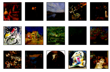
- # 绘图展示
- import matplotlib.pyplot as plt
- for i in range(15):
- plt.subplot(3,5,i+1)
- plt.imshow(sample[0][i]) #sample存放的是一个batch的图像
- plt.xticks([]) #不显示坐标刻度
- plt.yticks([])
- plt.show()
经过处理后的图像如下:
3. 网络构建
接下来到最重要的一步了,构建ResNet50网络,网络的结构图如下:resnet50结构图 ,可以根据这个结构图慢慢敲代码,我这里使用函数的方法构建ResNet50网络。ResNet的原理解释如下:六、ResNet网络详细解析(超详细哦)
- #(3)构建RNN-RESNET
- # conv_block部分
- def conv_block(input_tensor, filters, stride):
- # 分别接收卷积核的个数,即特征图的个数
- filter1, filter2, filter3 = filters
-
- # ==1== 正向传播部分
- # 卷积层
- x = layers.Conv2D(filter1, kernel_size=(1,1), strides=stride)(input_tensor)
- # BN层
- x = layers.BatchNormalization()(x)
- # 激活层
- x = layers.Activation('relu')(x)
-
- # 卷积层
- x = layers.Conv2D(filter2, kernel_size=(3,3), strides=(1,1), padding='same')(x)
- # BN层
- x = layers.BatchNormalization()(x)
- # 激活函数
- x = layers.Activation('relu')(x)
-
- # 卷积层
- x = layers.Conv2D(filter3, kernel_size=(1,1), strides=(1,1))(x)
- # BN层
- x = layers.BatchNormalization()(x)
-
- # ==2== shotcut部分
- # 卷积层
- shotcut = layers.Conv2D(filter3, kernel_size=(1,1), strides=stride)(input_tensor)
- # BN层
- shotcut = layers.BatchNormalization()(shotcut)
-
- # ==3== 两部分组合
- x = layers.add([x, shotcut])
- # 激活函数
- x = layers.Activation('relu')(x)
-
- # 返回结果
- return x
-
-
- # identity_block部分
- def iden_block(input_tensor, filters):
- # 接收卷积核的个数
- filter1, filter2, filter3 = filters
-
- # ==1== 正向传播
- # 卷积层
- x = layers.Conv2D(filter1, kernel_size=(1,1), strides=(1,1))(input_tensor)
- # BN层
- x = layers.BatchNormalization()(x)
- # 激活函数
- x = layers.Activation('relu')(x)
-
- # 卷积层
- x = layers.Conv2D(filter2, kernel_size=(3,3), strides=(1,1), padding='same')(x)
- # BN层
- x = layers.BatchNormalization()(x)
- # 激活函数
- x = layers.Activation('relu')(x)
-
- # 卷积层
- x = layers.Conv2D(filter3, kernel_size=(1,1), strides=(1,1))(x)
- # BN层
- x = layers.BatchNormalization()(x)
-
- # ==2== 结合
- x = layers.add([x, input_tensor])
- # 激活函数
- x = layers.Activation('relu')(x)
-
- return x
-
-
- # 本体
- def resnet50(input_shape=[224,224,3], output_shape=10):
- # 输入层
- inputs = keras.Input(shape=input_shape) #[224,224,3]
- # padding,上下左右各三层
- x = layers.ZeroPadding2D((3,3))(inputs)
-
- # 卷积层
- x = layers.Conv2D(64, kernel_size=(7,7), strides=(2,2))(x) #[112,112,64]
- # BN层
- x = layers.BatchNormalization()(x) #[112,112,64]
- # relu层
- x = layers.Activation('relu')(x) #[112,112,64]
- # 池化层
- x = layers.MaxPool2D(pool_size=(3,3), strides=(2,2))(x) #[55,55,64]
-
- # block1
- x = conv_block(x, [64, 64, 256], stride=(1,1)) #[55,55,256]
- x = iden_block(x, [64, 64, 256]) #[55,55,256]
- x = iden_block(x, [64, 64, 256]) #[55,55,256]
-
- # block2
- x = conv_block(x, [128, 128, 256], stride=(2,2)) #[28,28,512]
- x = iden_block(x, [128, 128, 256]) #[28,28,512]
- x = iden_block(x, [128, 128, 256]) #[28,28,512]
- x = iden_block(x, [128, 128, 256]) #[28,28,512]
-
- # block3
- x = conv_block(x, [256, 256, 1024], stride=(2,2)) #[14,14,1024]
- x = iden_block(x, [256, 256, 1024]) #[14,14,1024]
- x = iden_block(x, [256, 256, 1024]) #[14,14,1024]
- x = iden_block(x, [256, 256, 1024]) #[14,14,1024]
- x = iden_block(x, [256, 256, 1024]) #[14,14,1024]
- x = iden_block(x, [256, 256, 1024]) #[14,14,1024]
-
- # block4
- x = conv_block(x, [512, 512, 2048], stride=(2,2)) #[7,7,2048]
- x = iden_block(x, [512, 512, 2048]) #[7,7,2048]
- x = iden_block(x, [512, 512, 2048]) #[7,7,2048]
-
- # 平均池化层
- x = layers.AveragePooling2D(pool_size=(7,7))(x) #[1,1,2048]
- # Flatten层
- x = layers.Flatten()(x) #[None,2048]
- # 输出层,不做softmax
- outputs = layers.Dense(output_shape)(x)
-
- # 构建模型
- model = Model(inputs=inputs, outputs=outputs)
-
- # 返回模型
- return model
-
- # 创建restnet-50
- model = resnet50()
- # 查看网络结构
- model.summary()
网络结构如下
- __________________________________________________________________________________________________
- Layer (type) Output Shape Param # Connected to
- ==================================================================================================
- input_1 (InputLayer) [(None, 224, 224, 3 0 []
- )]
-
- zero_padding2d (ZeroPadding2D) (None, 230, 230, 3) 0 ['input_1[0][0]']
-
- conv2d (Conv2D) (None, 112, 112, 64 9472 ['zero_padding2d[0][0]']
- )
-
- batch_normalization (BatchNorm (None, 112, 112, 64 256 ['conv2d[0][0]']
- alization) )
-
- activation (Activation) (None, 112, 112, 64 0 ['batch_normalization[0][0]']
- )
-
-
- ----------------------------------------------------------------------------------------
- ----------------------------------------------------------------------------------------
- 省略N多层
- ----------------------------------------------------------------------------------------
- ----------------------------------------------------------------------------------------
-
-
- activation_48 (Activation) (None, 7, 7, 2048) 0 ['add_15[0][0]']
-
- activation_49 (Activation) (None, 7, 7, 2048) 0 ['activation_48[0][0]']
-
- average_pooling2d (AveragePool (None, 1, 1, 2048) 0 ['activation_49[0][0]']
- ing2D)
-
- flatten (Flatten) (None, 2048) 0 ['average_pooling2d[0][0]']
-
- dense (Dense) (None, 10) 20490 ['flatten[0][0]']
-
- ==================================================================================================
- Total params: 22,979,210
- Trainable params: 22,928,650
- Non-trainable params: 50,560
- __________________________________________________________________________________________________
4. 网络配置
采用动态学习率的方法,指定学习率是指数曲线下降,使网络刚开始时能更快接近最优点,后续再慢慢向逼近最优点。由于在网络的输出层没有进行softmax将实数值转为概率值,因此,在编译时使用交叉熵损失函数计算预测值和真实值的差异时,需要指定参数from_logits=True,代表将logits层输出的实数经过softmax转换为概率之后再和真实值计算损失。这样能有效提高数据稳定性。
- #(4)网络配置
- # 设置动态学习率
- exponential_decay = optimizers.schedules.ExponentialDecay(initial_learning_rate=0.0001, # 初始学习率
- decay_steps=2, # 衰减步长
- decay_rate=0.95) # 衰减率0.95
-
- # 编译
- model.compile(optimizer=optimizers.Adam(learning_rate=exponential_decay), #指定学习率
- #需要对真实值y进行onehot,而sparse_categorical_crossentropy会自动进行onehot
- loss = tf.losses.CategoricalCrossentropy(from_logits=True), # from_logits会自动将输出层的实数转为softmax后再计算交叉熵
- metrics = ['accuracy']) # 指定模型评价指标
-
- # 训练,给出训练集、验证集、循环10次、每轮循环开始之前重新洗牌
- model.fit(train_ds, validation_data=val_ds, epochs=10, shuffle=True)
5. 模型评估
绘制训练集和测试集的准确率和损失的对比曲线,观察是否出现过拟合现象。
- #(5)评估
- # ==1== 准确率
- train_acc = model.history['accuracy'] #训练集准确率
- val_acc = model.history['val_accuracy'] #验证集准确率
- # ==2== 损失
- train_loss = model.history['loss'] #训练集损失
- val_loss = model.history['val_loss'] #验证集损失
- # ==3== 绘图
- epochs_range = range(len(train_acc))
- plt.figure(figsize=(10,5))
- # 准确率
- plt.subplot(1,2,1)
- plt.plot(epochs_range, train_acc, label='train_acc')
- plt.plot(epochs_range, val_acc, label='val_acc')
- plt.legend()
- # 损失曲线
- plt.subplot(1,2,2)
- plt.plot(epochs_range, train_loss, label='train_loss')
- plt.plot(epochs_range, val_loss, label='val_loss')
- plt.legend()

