在GEE中使用S-G和Whittaker滤波_gee平滑处理

一套GEE数据插补平滑完整方案2：使用S-G和Whittaker滤波

KeyPoints

• 遥感数据缺失和平滑是一个问题。
• 数据缺失存在两种情况，一种是局部数据缺失，一种是整张影像缺失，影像后续分析。
• 数据平滑有助于去除噪声，使得数据更为清晰、准确。此外，遥感数据中常常包含着地形、云层等导致数据的波动较大，数据平滑可以改善图像质量。
• 对于数据处理，采取“先插补，再平滑”的策略。上期推文解决插补问题，这次解决平滑问题。
• 本文利用Savitzky-Golay滤波和Whittaker滤波解决上述两种情况。

S-G滤波

原理

S-G滤波（Savitzky-Golay滤波）是一种常用于数据平滑和拟合的数字滤波器。它可以在不降低信号分辨率的情况下去除信号中的噪声和粗糙部分，适用于各种数据类型，如光谱数据、生物信号、地球物理数据等。

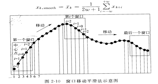
S-G滤波的原理是基于局部多项式拟合的思想，其核心是对信号进行局部加权多项式拟合。在滤波过程中，通过对一段信号进行多项式拟合，将该段信号近似为一个多项式函数。在拟合过程中，多项式的阶数和拟合窗口大小是两个关键参数，它们决定了拟合的复杂度和拟合的精度。一般来说，阶数和窗口大小应该根据数据的特征进行调整，以达到最佳的滤波效果。

S-G滤波可以通过矩阵运算的方式进行实现，这种方法计算速度较快，并且可以使用线性代数库来实现。S-G滤波常用于对光谱数据进行平滑处理，也可以用于对其他类型的数据进行平滑和去噪处理。

公式推导

以拟合一个三次多项式为例，窗口是5，根据三次多项式公式：

那么这五个窗口的值可以代入进去，写成矩阵形式：

不妨把上式写为：

那么我们只需要求解系数A，对应a0-a3，就能算出所有平滑的Y了，根据线性代数最小二乘的推导，A的解为：

只要在GEE函数中实现上述矩阵运算就行了

代码

第一步，加载数据

var geometry = /* color: #d63000 */ee.Geometry.Point([105.77243064871553, 13.54490072286009])
    
var filterLAI = function(img){
  var newimg = img.copyProperties(img, img.propertyNames());
  return newimg
}
var start_date = ee.Date('2019-09-27');
var end_date = ee.Date('2022-11-18'); 
var latter_lai = ee.ImageCollection('MODIS/006/MCD15A3H').select('Lai').filter(ee.Filter.date('2019-09-27', '2022-11-18')).map(filterLAI)
// getting rid of masked pixels
var latter_lai = latter_lai.map(function(img){return img.unmask(latter_lai.mean())});

/****************************************************************************
// Add predictors for SG fitting, using date difference
// We prepare for order 3 fitting, 
// but can be adapted to lower order fitting later on
****************************************************************************/
//to remove cloud

function mosaicByDate(imcol){
  // convert the ImageCollection into List
  var imlist = imcol.toList(imcol.size());
  // print(imlist)
  
  // Obtain the distinct image dates from the ImageCollection
  var unique_dates = imlist.map(function(im){
    return ee.Image(im).date().format("YYYY-MM-dd");
  }).distinct();
  // print(unique_dates);
  
  // mosaic the images acquired on the same date
  var mosaic_imlist = unique_dates.map(function(d){
    d = ee.Date(d);
    var im = imcol.filterDate(d, d.advance(1, "day")).mosaic();
    //print(im)
    // return the mosaiced same-date images and set the time properties
    return im.set(
      "system:time_start", d.millis(), 
      "system:id", d.format("YYYY-MM-dd")
      );
  });
  return ee.ImageCollection(mosaic_imlist);
} 

var modis_res =  latter_lai
                  .map(function(img){
                    var dstamp = ee.Date(img.get('system:time_start'));
                    var ddiff = dstamp.difference(ee.Date(start_date), 'day');
                    img = img.select(['Lai']).set('date', dstamp)
                            .clip(table).set('footprint',table);
                    return img.addBands(ee.Image(1).toFloat().rename('constant'))
                              .addBands(ee.Image(ddiff).toFloat().rename('t'))
                              .addBands(ee.Image(ddiff).pow(ee.Image(2)).toFloat().rename('t2'))
                              .addBands(ee.Image(ddiff).pow(ee.Image(3)).toFloat().rename('t3'));
                  });
print("modis_res",modis_res);
Map.addLayer(modis_res.max().select('Lai').clip(table),
            {'min':0,'max':30,'palette':['black','green']}, 'modis_res');
1

第二步，建立多项式：

这里设置window_size为9，多项式次数order为3，结合平滑效果请自行修改。

/****************************************************************************
// Step 2: Set up Savitzky-Golay smoothing
****************************************************************************/
// set the window size
var window_size = 9;
var half_window = (window_size - 1)/2;

// Define the axes of variation in the collection array.
var imageAxis = 0;
var bandAxis = 1;

// Set polynomial order
var order = 3;
var coeffFlattener = [['constant', 'x', 'x2', 'x3']];
var indepSelectors = ['constant', 't', 't2', 't3'];

// Convert the collection to an array.
var array = modis_res.toArray();

// For the remainder, use modis_res as a list of images
modis_res = modis_res.toList(modis_res.size());
var runLength = ee.List.sequence(0, modis_res.size().subtract(window_size));

// Run the SG solver over the series, and return the smoothed image version
var sg_series = runLength.map(function(i) {
  var ref = ee.Image(modis_res.get(ee.Number(i).add(half_window)));
  return getLocalFit(i).multiply(ref.select(indepSelectors))
                      .reduce(ee.Reducer.sum()).copyProperties(ref);
});
print("sg_series",sg_series);
1

第三步，求解，利用matrixSolve求解矩阵

// Solve 
function getLocalFit(i){
  // Get a slice corresponding to the window_size of the SG smoother
  var subarray = array.arraySlice(imageAxis, ee.Number(i).int(), ee.Number(i).add(window_size).int());
  var predictors = subarray.arraySlice(bandAxis, 1, 1 + order + 1);
  var response = subarray.arraySlice(bandAxis, 0, 1); // NDVI
  var coeff = predictors.matrixSolve(response);
  coeff = coeff.arrayProject([0]).arrayFlatten(coeffFlattener);
  return coeff;  
}
1

第四步，根据求解多项式的系数，生成结果：

// Part 3: Generate some output
// 3A. Get an example original image and its SG-ed version
var NDVI = (ee.Image(modis_res.get(50)).select('Lai'));
var NDVIsg = (ee.Image(sg_series.get(50)));  // half-window difference in index
Map.addLayer(NDVI,{min:0,max:30},"NDVI");
Map.addLayer(NDVIsg,{min:0,max:30},"NDVIsg");
1

最后结果如图所示：

完整的代码可以后台回复获取，见后文

Whittaker滤波

原理

Whittaker滤波是一种基于时间序列的平滑方法，通过对时间序列进行加权平均来平滑信号。其原理基于以下两个假设：

1. 时间序列中的数据点存在一个随机误差，该误差是服从正态分布的，并且误差是独立同分布的。
2. 时间序列中数据点之间并没有显著的周期性或趋势性变化。

Whittaker滤波的核心思想是对每个数据点进行加权平均，权重系数是根据时间和空间距离计算的。具体来说，Whittaker滤波算法将每个数据点表示为一个二维网格（即空间-时间网格），并且使用高斯核函数来计算每个数据点在该网格内的权重。然后，通过加权平均来计算每个数据点的平滑值。

Whittaker滤波可以应用于多种不同类型的时间序列数据，包括光谱数据、图像数据和地理空间数据等。它被广泛应用于信号处理、数据降噪和数据插值等领域。

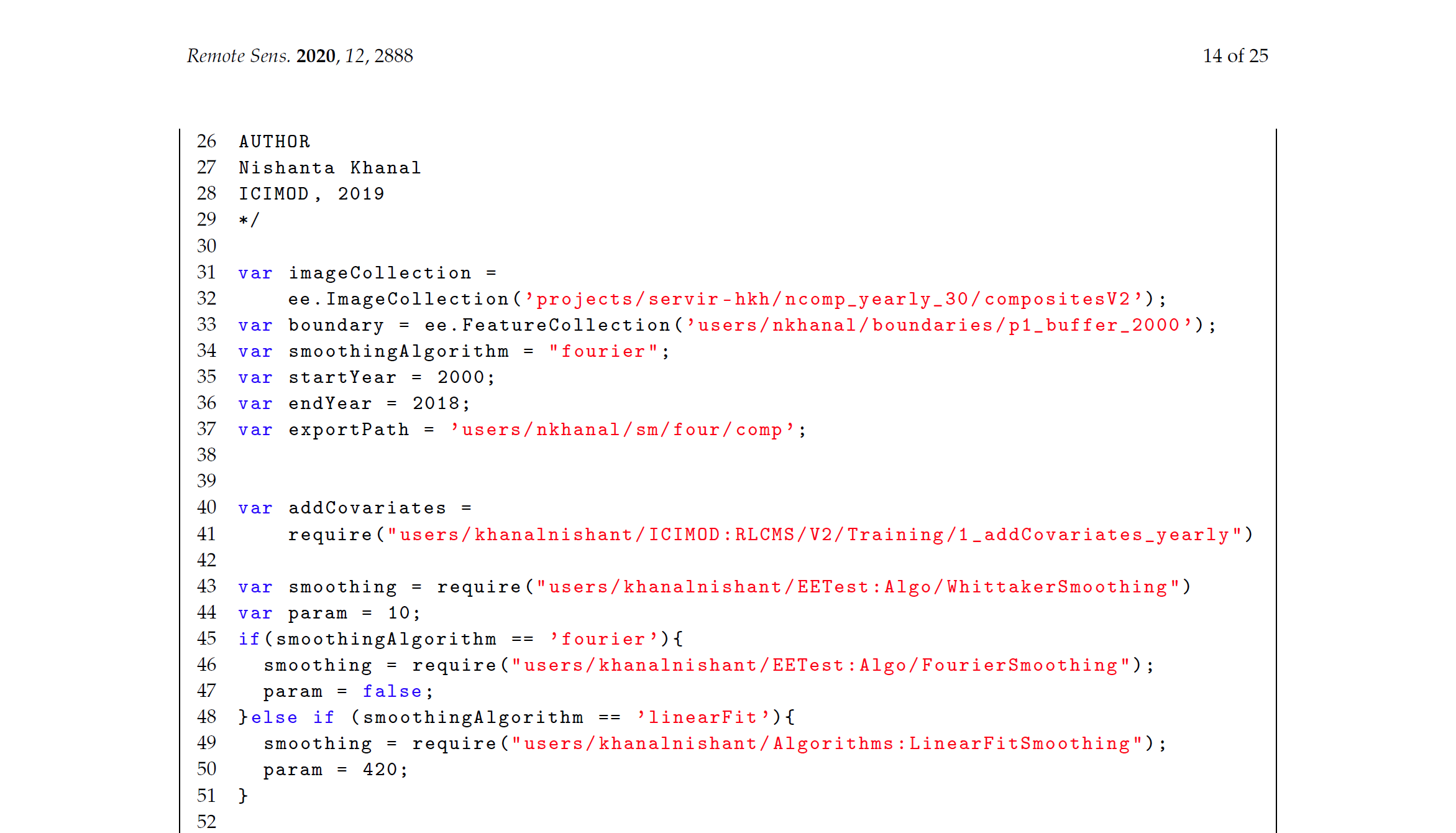
根据Nishanta等人发表在Remote Sensing上的文章：

Whittaker能用于GEE，并产生比SG更好的效果

代码

Nishanta等人在论文附录公布了代码，然而他的代码只是对于土地覆盖，因此对其进行了一些修改，使之适用于NDVI、LAI等变量：

由于篇幅有限，这里不再展示完整代码，仅展示结果：

S-G与Whittaker对比

可以看到Whittaker滤波总体上比三次多项式S-G好。

在细节信息上，S-G能较大程度保留一些细节信号（但这些细节信号更有可能是异常信号，如云量，噪声等等），反而产生错误的结果。

在遥感数据，植被信号等，Whittaker滤波可能比S-G滤波更适合。

Whittaker通过对原始数据进行重构来消除噪声和不规则性。它的效果通常取决于所选择的平滑因子和曲线拟合程度。

与之相比，S-G滤波是使用多项式拟合来平滑信号，并且可以控制拟合的阶数和窗口大小，该方法较为粗糙。

最近越来越多研究也关注改进后的Whittaker滤波，而很少用S-G处理这些遥感信号。

如Kong等人发表在ISPRS的研究，提出了一种加权后的Whittaker方法，并在空间尺度上设置动态参数lambda（称为wWHd方法）。显著改善了精度。

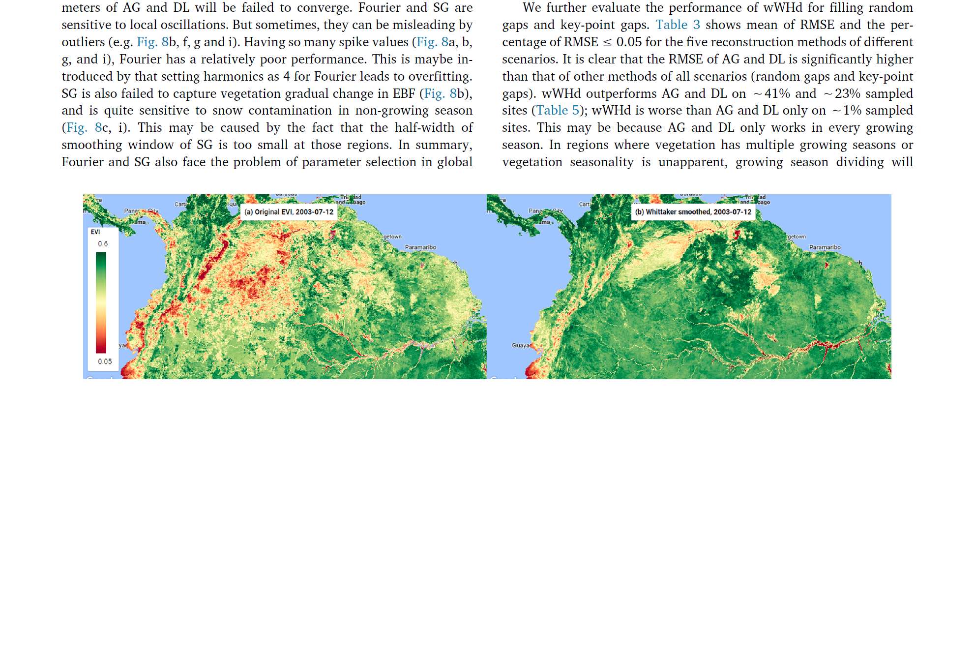
效果如图：

如有相关需求，可以引用系列文章：

Kong, D., Zhang, Y., Gu, X., & Wang, D. (2019). A robust method for reconstructing global MODIS EVI time series on the Google Earth Engine. ISPRS Journal of Photogrammetry and Remote Sensing, 155, 13-24.

Kong, D., McVicar, T. R., Xiao, M., Zhang, Y., Peña‐Arancibia, J. L., Filippa, G., ... & Gu, X. (2022). phenofit: An R package for extracting vegetation phenology from time series remote sensing. Methods in Ecology and Evolution, 13(7), 1508-1527.

代码

上述S-G代码和Whittaker代码可以后台回复【GEE滤波】，wWHd相关请参考孔老师GitHub，wWHd：https://github.com/gee-hydro/gee_whittaker

S-G：https://code.earthengine.google.com/c73b17534179363adb578558d46f78a7

Whittaker：https://code.earthengine.google.com/67448f422e8a55132e87cff1653a67ee