卡尔曼滤波— Constant Velocity Model

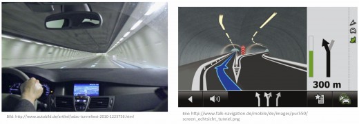
假设你开车进入隧道，GPS信号丢失，现在我们要确定汽车在隧道内的位置。汽车的绝对速度可以通过车轮转速计算得到，汽车朝向可以通过yaw rate sensor(A yaw-rate sensor is a gyroscopic device that measures a vehicle’s angular velocity around its vertical axis. )得到，因此可以获得X轴和Y轴速度分量Vx，Vy

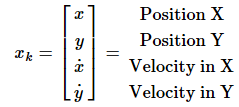
首先确定状态变量，恒速度模型中取状态变量为汽车位置和速度：

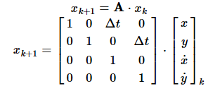
根据运动学定律(The basic idea of any motion models is that a mass cannot move arbitrarily due to inertia)：

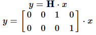
由于GPS信号丢失，不能直接测量汽车位置，则观测模型为：

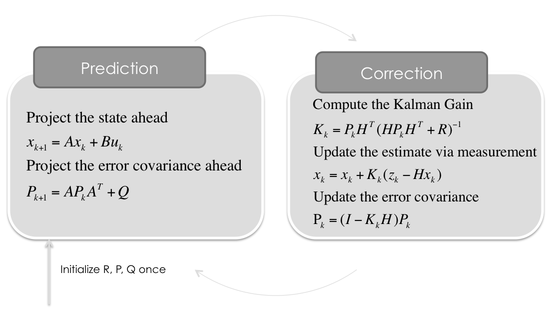
卡尔曼滤波步骤如下图所示：

# -*- coding: utf-8 -*-
import numpy as np
import matplotlib.pyplot as plt

# Initial State x0
x = np.matrix([[0.0, 0.0, 0.0, 0.0]]).T

# Initial Uncertainty P0
P = np.diag([1000.0, 1000.0, 1000.0, 1000.0])

dt = 0.1 # Time Step between Filter Steps

# Dynamic Matrix A
A = np.matrix([[1.0, 0.0, dt, 0.0],
              [0.0, 1.0, 0.0, dt],
              [0.0, 0.0, 1.0, 0.0],
              [0.0, 0.0, 0.0, 1.0]])

# Measurement Matrix
# We directly measure the velocity vx and vy
H = np.matrix([[0.0, 0.0, 1.0, 0.0],
              [0.0, 0.0, 0.0, 1.0]])

# Measurement Noise Covariance
ra = 10.0**2
R = np.matrix([[ra, 0.0],
              [0.0, ra]])

# Process Noise Covariance
# The Position of the car can be influenced by a force (e.g. wind), which leads
# to an acceleration disturbance (noise). This process noise has to be modeled
# with the process noise covariance matrix Q.
sv = 8.8
G = np.matrix([[0.5*dt**2],
               [0.5*dt**2],
               [dt],
               [dt]])
Q = G*G.T*sv**2

I = np.eye(4)

# Measurement
m = 200 # 200个测量点
vx= 20  # in X
vy= 10  # in Y
mx = np.array(vx+np.random.randn(m))
my = np.array(vy+np.random.randn(m))
measurements = np.vstack((mx,my))

# Preallocation for Plotting
xt = []
yt = []


# Kalman Filter
for n in range(len(measurements[0])):
    
    # Time Update (Prediction)
    # ========================
    # Project the state ahead
    x = A*x
    
    # Project the error covariance ahead
    P = A*P*A.T + Q

    
    # Measurement Update (Correction)
    # ===============================
    # Compute the Kalman Gain
    S = H*P*H.T + R
    K = (P*H.T) * np.linalg.pinv(S)

    # Update the estimate via z
    Z = measurements[:,n].reshape(2,1)
    y = Z - (H*x)                            # Innovation or Residual
    x = x + (K*y)
    
    # Update the error covariance
    P = (I - (K*H))*P

    
    # Save states for Plotting
    xt.append(float(x[0]))
    yt.append(float(x[1]))


# State Estimate: Position (x,y)
fig = plt.figure(figsize=(16,16))
plt.scatter(xt,yt, s=20, label='State', c='k')
plt.scatter(xt[0],yt[0], s=100, label='Start', c='g')
plt.scatter(xt[-1],yt[-1], s=100, label='Goal', c='r')

plt.xlabel('X')
plt.ylabel('Y')
plt.title('Position')
plt.legend(loc='best')
plt.axis('equal')
plt.show()

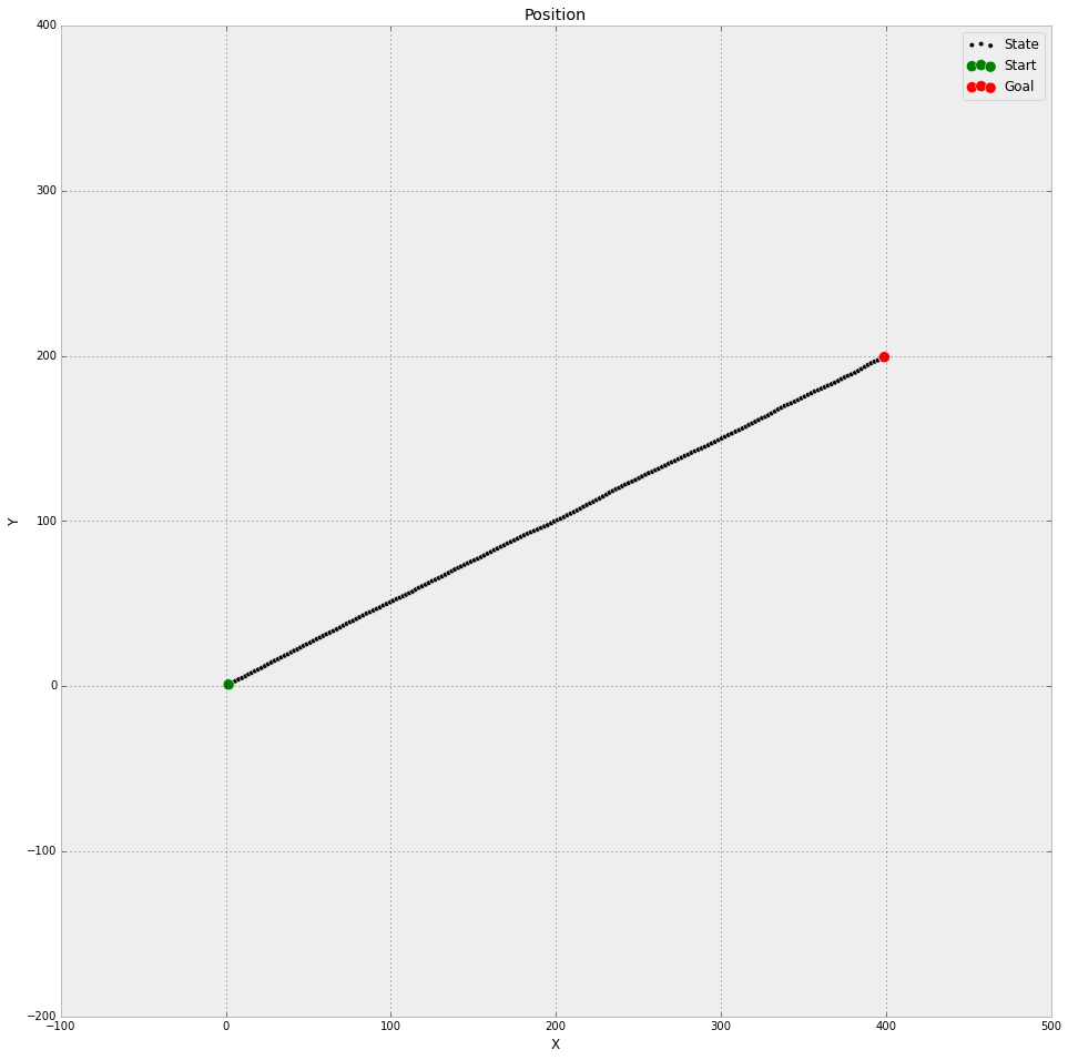
汽车在隧道中的估计位置如下图：

 

 参考

Improving IMU attitude estimates with velocity data

https://zhuanlan.zhihu.com/p/25598462