
- 1微信小程序:实现音乐播放器的功能_this.data.audiocontext.play()
- 2vue滚动加载列表数据展示封装懒加载_vue 滚动加载数据
- 3Vue3 实现滚动加载更多_vue3 如何实现滚动加载
- 4Kafka 生产者_kafka多个生产者
- 5H5网页使用支付宝授权登录获取用户信息详解_alipay.system.oauth.token
- 6spark编程实战(四) —— 词频统计(WordCount)和 Top K_spark统计以上5个文件中的单词词频(wordcount),结果保存到hdfs中,截图频率最高的5
- 7docker ui 部署_docker x-ui
- 8机器学习集成学习与模型融合!
- 9堆排序算法(图解详细流程)
- 10mac photoshop install无法安装_MAC安装软件显示‘无法确认安全’或‘将其移至废纸篓’解决办法...
Tensorflow2.0之神经风格迁移
赞
踩
什么是神经风格迁移
此文章使用深度学习来用其他图像的风格创造一个图像。 这被称为神经风格迁移。
神经风格迁移是一种优化技术,用于将两个图像(一个内容图像和一个风格参考图像)混合在一起,使输出的图像看起来像内容图像, 但是使用了风格参考图像的风格。
这是通过优化输出图像以匹配内容图像的内容统计数据和风格参考图像的风格统计数据来实现的。 这些统计数据可以使用卷积网络从图像中提取。
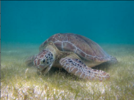
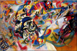
如左图为内容图片,右图为风格图片。
那么在进行完风格迁移之后,我们应该得到类似下图的图片。

代码实现
1、导入需要的库
import tensorflow as tf
import IPython.display as display
import numpy as np
import matplotlib.pyplot as plt
import matplotlib as mpl
mpl.rcParams['figure.figsize'] = (12,12)
mpl.rcParams['axes.grid'] = False
- 1
- 2
- 3
- 4
- 5
- 6
- 7
2、下载图片
content_path = tf.keras.utils.get_file('turtle.jpg','https://storage.googleapis.com/download.tensorflow.org/example_images/Green_Sea_Turtle_grazing_seagrass.jpg')
style_path = tf.keras.utils.get_file('kandinsky.jpg','https://storage.googleapis.com/download.tensorflow.org/example_images/Vassily_Kandinsky%2C_1913_-_Composition_7.jpg')
- 1
- 2
上面代码得到的是两张图片的存储路径。
3、将图片加载到程序中
def load_img(path_to_img):
    max_dim = 512
    img = tf.io.read_file(path_to_img)
    img = tf.image.decode_image(img, channels=3)
    img = tf.image.convert_image_dtype(img, tf.float32)

    shape = tf.cast(tf.shape(img)[:-1], tf.float32)
    long_dim = max(shape)
    scale = max_dim / long_dim

    new_shape = tf.cast(shape*scale, tf.int32)

    img = tf.image.resize(img, new_shape)
    img = img[tf.newaxis, :]
    return img

content_image = load_img(content_path)
style_image = load_img(style_path)
# 绘图函数
def imshow(image, title=None):
    if len(image.shape) > 3:
        image = tf.squeeze(image, axis=0)

    plt.imshow(image)
    if title:
        plt.title(title)

- 1
- 2
- 3
- 4
- 5
- 6
- 7
- 8
- 9
- 10
- 11
- 12
- 13
- 14
- 15
- 16
- 17
- 18
- 19
- 20
- 21
- 22
- 23
- 24
- 25
- 26
上述代码中:
img = tf.io.read_file(path_to_img) 将图片加载到程序中,但此时得到的img是经编码后的,我们并不能明白它代表什么。
img = tf.image.decode_image(img, channels=3) 将加载的图片解码成像素值数组。
img = tf.image.convert_image_dtype(img, tf.float32) 将所有图片像素同除255,并将该数组数据设置为浮点型。
其余部分的目的是将图片的长宽等比例缩放成使其最长边等于512。
4、加载VGG19模型,并打印出其中所有的层
vgg = tf.keras.applications.VGG19(include_top=False, weights='imagenet')

for layer in vgg.layers:
    print(layer.name)
- 1
- 2
- 3
- 4
input_1
block1_conv1
block1_conv2
block1_pool
block2_conv1
block2_conv2
block2_pool
block3_conv1
block3_conv2
block3_conv3
block3_conv4
block3_pool
block4_conv1
block4_conv2
block4_conv3
block4_conv4
block4_pool
block5_conv1
block5_conv2
block5_conv3
block5_conv4
block5_pool
- 1
- 2
- 3
- 4
- 5
- 6
- 7
- 8
- 9
- 10
- 11
- 12
- 13
- 14
- 15
- 16
- 17
- 18
- 19
- 20
- 21
- 22
5、从VGG19中挑出风格层和内容层
风格层的输出旨在代表风格图片的特征,内容层的输出旨在表示内容图片的特征。
content_layers = ['block5_conv2']
style_layers = ['block1_conv1',
                'block2_conv1',
                'block3_conv1',
                'block4_conv1',
                'block5_conv1']

num_content_layers = len(content_layers)
num_style_layers = len(style_layers)
- 1
- 2
- 3
- 4
- 5
- 6
- 7
- 8
- 9
6、改变VGG19模型
因为原始的VGG19模型输出分类结果(概率),但在风格迁移时我们需要的是两张图片各自的特征,即不同层的输出,所以要重新对VGG19的输出进行定义。
def vgg_layers(layer_names):
    """ Creates a vgg model that returns a list of intermediate output values."""
    # 加载我们的模型。 加载已经在 imagenet 数据上预训练的 VGG
    vgg = tf.keras.applications.VGG19(include_top=False, weights='imagenet')
    vgg.trainable = False

    outputs = [vgg.get_layer(name).output for name in layer_names]

    model = tf.keras.Model([vgg.input], outputs)
    return model
- 1
- 2
- 3
- 4
- 5
- 6
- 7
- 8
- 9
- 10
此处详解参考Tensorflow2.0如何在网络中规定多个输出。
7、风格计算
图像的风格可以通过不同风格层的输出的平均值和相关性来描述。 通过在每个位置计算这些输出向量的外积,并在所有位置对该外积进行平均,可以计算出包含此信息的 Gram 矩阵。 对于特定层的 Gram 矩阵,具体计算方法如下所示:

上式中的
l
,
i
,
j
,
c
,
d
l,i,j,c,d
l,i,j,c,d可以这样解释:
我们知道,输入神经网络的一张图片的形状应该类似这种形式:[1, 256, 128, 3]。那么
l
l
l表示第几张图片,这里为1;
i
i
i表示256;
j
j
j 表示128;
c
c
c和
d
d
d都等于3(因为是同一张图片,所以
c
=
d
c=d
c=d)。
def gram_matrix(input_tensor):
    result = tf.linalg.einsum('bijc,bijd->bcd', input_tensor, input_tensor)
    input_shape = tf.shape(input_tensor)
    num_locations = tf.cast(input_shape[1]*input_shape[2], tf.float32)
    return result/(num_locations)
- 1
- 2
- 3
- 4
- 5
其中,tf.linalg.einsum(‘bijc,bijd->bcd’, input_tensor, input_tensor) 旨在计算Gram矩阵。其详细说明请参考:tf.linalg.einsum。
8、建立风格迁移模型
class StyleContentModel(tf.keras.models.Model):
    def __init__(self, style_layers, content_layers):
        super(StyleContentModel, self).__init__()
        self.vgg =  vgg_layers(style_layers + content_layers)
        self.style_layers = style_layers
        self.content_layers = content_layers
        self.num_style_layers = len(style_layers)
        self.vgg.trainable = False

    def call(self, inputs):
        "Expects float input in [0,1]"
        inputs = inputs*255.0
        preprocessed_input = tf.keras.applications.vgg19.preprocess_input(inputs)
        outputs = self.vgg(preprocessed_input)
        style_outputs, content_outputs = (outputs[:self.num_style_layers],
                                          outputs[self.num_style_layers:])

        style_outputs = [gram_matrix(style_output)
                         for style_output in style_outputs]

        content_dict = {content_name:value
                        for content_name, value
                        in zip(self.content_layers, content_outputs)}

        style_dict = {style_name:value
                      for style_name, value
                      in zip(self.style_layers, style_outputs)}

        return {'content':content_dict, 'style':style_dict}

extractor = StyleContentModel(style_layers, content_layers)
- 1
- 2
- 3
- 4
- 5
- 6
- 7
- 8
- 9
- 10
- 11
- 12
- 13
- 14
- 15
- 16
- 17
- 18
- 19
- 20
- 21
- 22
- 23
- 24
- 25
- 26
- 27
- 28
- 29
- 30
- 31
实例化此模型时,其输入为风格层和内容层。将图片输入此模型后,得到一个字典,包含 ‘content’ 和 ‘style’ ,分别表示风格层的输出(五层输出)和内容层的输出(一层输出)。
9、得到风格图片的风格特征和内容图片的内容特征
将风格图片和内容图片分别输入模型,分别取其风格特征和内容特征。
style_targets = extractor(style_image)['style']
content_targets = extractor(content_image)['content']
- 1
- 2
10、将内容图片设置为变量
因为输入的内容图片不断地改变其风格直到接近风格图片的风格,所以定义一个 tf.Variable 来表示要优化的图像。
image = tf.Variable(content_image)
- 1
11、定义优化函数
opt = tf.optimizers.Adam(learning_rate=0.02, beta_1=0.99, epsilon=1e-1)
- 1
12、定义损失函数
style_weight = 1e-2
content_weight = 1e4

def style_content_loss(outputs):
    style_outputs = outputs['style']
    content_outputs = outputs['content']
    # 计算风格损失
    style_loss = tf.add_n([tf.reduce_mean((style_outputs[name]-style_targets[name])**2)
                           for name in style_outputs.keys()])
    style_loss *= style_weight / num_style_layers
	# 计算内容损失
    content_loss = tf.add_n([tf.reduce_mean((content_outputs[name]-content_targets[name])**2)
                             for name in content_outputs.keys()])
    content_loss *= content_weight / num_content_layers
    # 计算总损失
    loss = style_loss + content_loss
    return loss
- 1
- 2
- 3
- 4
- 5
- 6
- 7
- 8
- 9
- 10
- 11
- 12
- 13
- 14
- 15
- 16
- 17
style_weight 和content_weight 分别表示风格上的损失和内容上的损失在计算总损失时所占的比重。
13、定义每一步的梯度下降
首先,由于这是一个浮点图像,因此我们需要定义一个函数来保持像素值保持在 0 和 1 之间:
def clip_0_1(image):
    return tf.clip_by_value(image, clip_value_min=0.0, clip_value_max=1.0)
- 1
- 2
然后,通过梯度带来进行参数优化。
@tf.function()
def train_step(image):
    with tf.GradientTape() as tape:
        outputs = extractor(image)
        loss = style_content_loss(outputs)

    grad = tape.gradient(loss, image)
    opt.apply_gradients([(grad, image)])
    image.assign(clip_0_1(image))
- 1
- 2
- 3
- 4
- 5
- 6
- 7
- 8
- 9
有关梯度带的详细信息可以参考:Tensorflow2.0中的梯度带(GradientTape)以及梯度更新。
14、训练模型,优化图片
epochs = 10
steps_per_epoch = 100

step = 0
for n in range(epochs):
    for m in range(steps_per_epoch):
        step += 1
        train_step(image)
        print(".", end='')
    display.clear_output(wait=True)
    imshow(image.read_value())
    plt.title("Train step: {}".format(step))
    plt.show()
- 1
- 2
- 3
- 4
- 5
- 6
- 7
- 8
- 9
- 10
- 11
- 12
- 13
迭代1000次之后,得到图片:

15、总变分损失
此实现只是一个基础版本,它的一个缺点是它会产生大量的高频误差。 我们可以直接通过正则化图像的高频分量来减少这些高频误差。 在风格转移中,这通常被称为总变分损失。
计算高频分量
本质上高频分量是一个边缘检测器,我们可以定义一个函数得到图片的高频分量。
def high_pass_x_y(image):
    x_var = image[:,:,1:,:] - image[:,:,:-1,:]
    y_var = image[:,1:,:,:] - image[:,:-1,:,:]

    return x_var, y_var
- 1
- 2
- 3
- 4
- 5
我们可以将图片的高频分量显示出来:
x_deltas, y_deltas = high_pass_x_y(content_image)

plt.figure(figsize=(14,10))
plt.subplot(2,2,1)
imshow(clip_0_1(2*y_deltas+0.5), "Horizontal Deltas: Original")

plt.subplot(2,2,2)
imshow(clip_0_1(2*x_deltas+0.5), "Vertical Deltas: Original")

x_deltas, y_deltas = high_pass_x_y(image)

plt.subplot(2,2,3)
imshow(clip_0_1(2*y_deltas+0.5), "Horizontal Deltas: Styled")

plt.subplot(2,2,4)
imshow(clip_0_1(2*x_deltas+0.5), "Vertical Deltas: Styled")
- 1
- 2
- 3
- 4
- 5
- 6
- 7
- 8
- 9
- 10
- 11
- 12
- 13
- 14
- 15
- 16

计算总变分损失
def total_variation_loss(image):
    x_deltas, y_deltas = high_pass_x_y(image)
    return tf.reduce_mean(x_deltas**2) + tf.reduce_mean(y_deltas**2)
- 1
- 2
- 3
16、将总变分损失计入总损失
total_variation_weight=1e8

@tf.function()
def train_step(image):
    with tf.GradientTape() as tape:
        outputs = extractor(image)
        loss = style_content_loss(outputs)
        loss += total_variation_weight*total_variation_loss(image)

    grad = tape.gradient(loss, image)
    opt.apply_gradients([(grad, image)])
    image.assign(clip_0_1(image))
- 1
- 2
- 3
- 4
- 5
- 6
- 7
- 8
- 9
- 10
- 11
- 12
17、重新训练模型
image = tf.Variable(content_image)

epochs = 10
steps_per_epoch = 100

step = 0
for n in range(epochs):
    for m in range(steps_per_epoch):
        step += 1
        train_step(image)
        print(".", end='')
    display.clear_output(wait=True)
    imshow(image.read_value())
    plt.title("Train step: {}".format(step))
    plt.show()
- 1
- 2
- 3
- 4
- 5
- 6
- 7
- 8
- 9
- 10
- 11
- 12
- 13
- 14
- 15

【注】有需要源码的小伙伴请戳:Tensorflow2.0之神经风格迁移


