语义分割空间上下文关系_多尺度空间注意的语义分割

This blog presents a novel neural network using multi scale feature fusion at different scales for accurate and efficient semantic segmentation.

该博客介绍了一种新颖的神经网络，该网络使用不同尺度的多尺度特征融合来进行准确有效的语义分割。

重要事项 (Important Points)

1. We have used dilated convolutional layers in downsampling part, transposed convolutional layers in the upsampling part and concat layers to merge them.
   我们在下采样部分中使用了膨胀的卷积层，在上采样部分中使用了转置的卷积层，并使用concat层将它们合并。
2. Skip connections in between alternate blocks are used which helps in reducing overfitting considerably.
   在备用块之间使用了跳过连接，这有助于显着减少过拟合。
3. We present an in depth theoretical analysis of our network with training and optimization details.
   我们对网络进行了深入的理论分析，并提供了培训和优化方面的详细信息。
4. We evaluated our network on the Camvid dataset using mean accuracy per class and Intersection Over Union (IOU) as the evaluation metrics.
   我们使用每类的平均准确性和“交叉口交集”(IOU)作为评估指标，在Camvid数据集上评估了我们的网络。
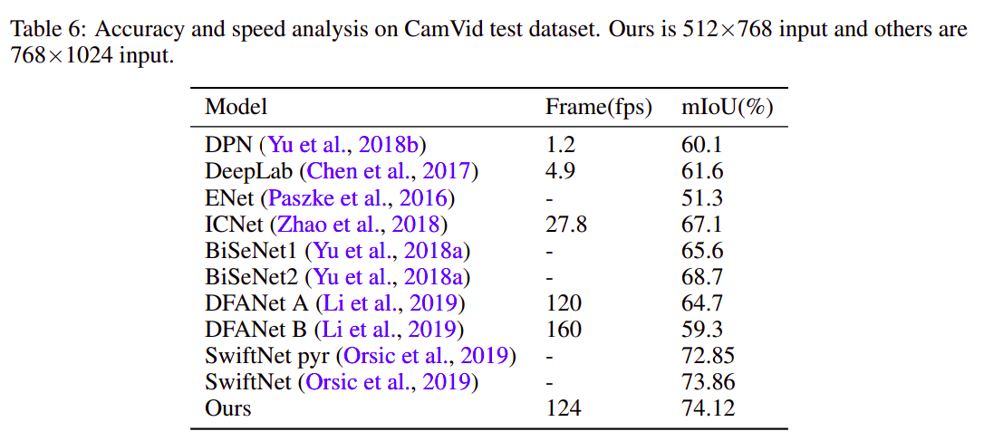
5. Our model outperforms previous state of the art networks on semantic segmentation achieving mean IOU value of 74.12 while running at >100 FPS.
   我们的模型在语义分割方面优于先前的现有技术网络，在> 100 FPS上运行时达到了平均IOU值74.12。

语义分割 (Semantic Segmentation)

Semantic segmentation requires predicting a class for each and every pixel of the input image, instead of only discrete classes for the whole input images. In order to predict what is present in the image for each and every pixel, segmentation needs to find not only what is in the input image, but also where it is. The applications of semantic segmentation autonomous driving, video surveillance, medical imaging etc. This is a challenging problem as there is a tradeoff between accuracy and speed. Since the model eventually needs to be deployed in real world setting, both accuracy and speed should be high.

语义分割需要为输入图像的每个像素预测一个类，而不是为整个输入图像仅预测一个离散类。 为了预测每个像素中图像中存在的内容，分割不仅需要找到输入图像中的内容，还需要找到它的位置。 语义分段自动驾驶，视频监视，医学成像等的应用。这是一个具有挑战性的问题，因为需要在准确性和速度之间进行权衡。 由于模型最终需要在实际环境中部署，因此准确性和速度都应该很高。

数据集 (Dataset)

For training and evaluation, Cambridge-driving Labeled Video Database (CamVid) dataset is used. The database provides ground truth labels that associate each pixel with one of 32 classes. The images are of size 360×480. A sample ground truth image from dataset is shown in Fig 1:

为了进行培训和评估，使用了剑桥驾驶标签视频数据库(CamVid)数据集。 该数据库提供了将每个像素与32个类别之一相关联的地面真相标签。 图像尺寸为360×480。 来自数据集的样本地面真相图像如图1所示：

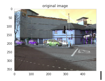
The original images are taken as ground truth. For any algorithm, the metrics are always evaluated in comparison to the ground truth data. The ground truth information is provided in the dataset for the training and test set. For semantic segmentation problems, the ground truth includes the image, the classes of the objects in it and a segmentation mask for each and every object present in a particular image. These images are shown in binary format for each of the twelve classes separately in Fig 2:

原始图像被当作地面真理。 对于任何算法，始终将评估指标与真实情况数据进行比较。 在训练和测试集的数据集中提供了地面真相信息。 对于语义分割问题，基本事实包括图像，其中的对象类别以及特定图像中存在的每个对象的分割蒙版。 这些图像分别以二进制格式显示了十二个类别中的每一个类别：

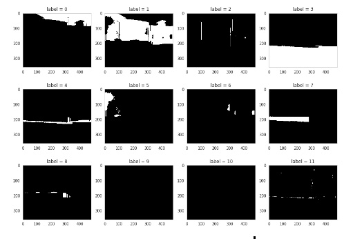
The classes are Sky, Building, Pole, Road, Pavement, Tree, SignSymbol, Fence, Car, Pedestrian and Bicyclist.

这些类别包括天空，建筑物，杆，道路，人行道，树木，SignSymbol，栅栏，汽车，行人和自行车。

网络架构 (Network Architecture)

The network architecture is explained in the following points:

以下几点说明了网络体系结构：

1. We resized the images to 224×224 pixels which was originally at 360×480 pixels.
   我们将图像的大小调整为224×224像素，最初为360×480像素。
2. We split the dataset into 2 parts with 85 percent images in the training set and 15 percent images in the test set.
   我们将数据集分为两部分，训练集中的图像占85％，测试集中的图像占15％。
3. The loss function used is categorical cross entropy.
   所使用的损失函数是分类交叉熵。
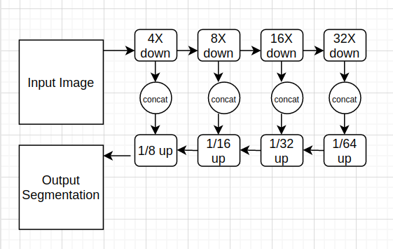
4. We used dilated convolution in place of normal convolution layers in downsampling layers which are used for reducing the feature maps and transposed convolution in place of normal convolution layers in upsampling layers to recover the features back.
   我们在下采样层中使用膨胀卷积代替了常规卷积层，用于缩小特征图，并在上采样层中使用了转置卷积代替了常规卷积层以恢复特征。
5. We used concat operation in between the layers to merge the features at different scales.
   我们在层之间使用了concat操作来合并不同比例的要素。
6. For the convolutional layer we didn’t use any padding, used 3×3 filter and use relu as the activation function. For the max pooling layer, we used 2×2 filters and strides of 2×2.
   对于卷积层，我们不使用任何填充，使用3×3滤镜，并使用relu作为激活函数。 对于最大池化层，我们使用2×2过滤器，步幅为2×2。
7. We used VGG16 as the pre trained backbone for training the model.
   我们使用VGG16作为训练模型的预训练骨干。
8. Softmax is used as the activation function in the last layer to output discrete probabilities of whether an object is present in a particular pixel location or not.
   Softmax在最后一层用作激活函数，以输出对象是否存在于特定像素位置中的离散概率。
9. We used Adam as the optimizer.
   我们使用亚当作为优化器。
10. The batch size value of 4 was used which we found to be optimal to avoid overfitting.
    批次大小值为4，我们发现这是避免过度拟合的最佳选择。

The network architecture used in this work is shown in Fig 3:

这项工作中使用的网络架构如图3所示：

优化 (Optimization)

Suppose given a local feature C, we feed it into a convolution layers to generate two new feature maps B and C respectively. We perform a matrix multiplication between the transpose of A and B, and apply a softmax layer to calculate the spatial attention map as defined in the equation below:

假设给定了局部特征C，我们将其馈入卷积层以分别生成两个新的特征图B和C。 我们在A和B的转置之间执行矩阵乘法，并应用softmax层来计算空间注意图，如以下等式中所定义：

We perform a matrix multiplication between the transpose of X and A and reshape their results. Then we multiply the result by a scale parameter β and perform an element-wise sum operation with A to obtain the final output as shown in the equation below:

我们在X和A的转置之间执行矩阵乘法，并对它们的结果进行整形。 然后，将结果与比例参数β相乘，并用A进行逐元素求和运算，以得到最终输出，如下式所示：

The above equation shows that the resultant feature of each channel is a weighted sum of the features of all channels and models the semantic dependencies between feature maps at various scales. For a single backbone, a stage process, the stage in the previous backbone network and sub-stage aggregation method can be formulated as shown in the equation below:

上面的等式表明，每个通道的合成特征是所有通道的特征的加权总和，并以各种比例对特征图之间的语义依赖性进行建模。 对于单个骨干，可以按照以下等式来制定阶段过程，先前的骨干网络中的阶段和子阶段聚合方法：

Here i refers to the index of the stage.

我在这里指的是阶段的索引。

实验 (Experiments)

The effect of the number of pooling layers on Intersection Over Union(IOU) is shown in Table 2.

表2中显示了合并层数对“相交越界”(IOU)的影响。

The effect of varying the number of branches and fusion methods used in model architecture on IOU is shown in Table 3.

表3显示了更改模型架构中使用的分支数量和融合方法对IOU的影响。

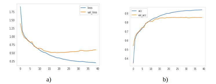
The model is trained for 40 epochs, training mean pixel accuracy of 93 percent and validation mean pixel accuracy of 88 percent is achieved. The loss and pixel wise accuracy (both training and test) are plotted as a function of epochs in Fig 4:

该模型经过40个时期的训练，训练的平均像素精度为93％，验证的平均像素精度为88％。 损耗和像素精度(训练和测试)均作为历元的函数绘制在图4中：

评估指标 (Evaluation Metrics)

For evaluation, the following two metrics were used:

为了进行评估，使用了以下两个指标：

1. Mean Accuracy per-class — This metric outputs the class wise prediction accuracy per pixel.

1.每个类别的平均准确度-此度量标准输出每个像素的逐级预测准确度。

2. Mean IOU — It is a segmentation performance parameter that measures the overlap between two objects by calculating the ratio of intersection and union with ground truth masks.

2.平均IOU —这是一种分割性能参数，通过计算与地面真值蒙版的交集和并集的比率来测量两个对象之间的重叠。

The class wise IOU values were calculated using the equation below.

使用以下等式计算逐级IOU值。

Where TP denotes true positive, FP denotes false positive, FN denotes false negative and IOU denotes Intersection over union value.

其中TP表示真阳性，FP表示假阳性，FN表示假阴性，IOU表示联合值的交集。

结果 (Results)

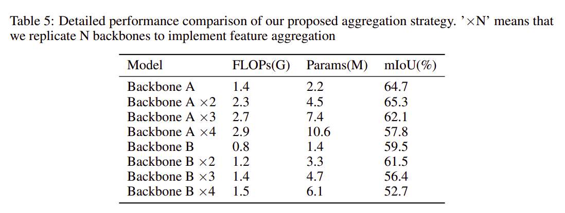
The effect of using multiple blocks, FLOPS and parameters on IOU is shown in Table 5. Here FLOPS and parameters are a measure of computation required by our model architecture.

表5显示了在IOU上使用多个块，FLOPS和参数的效果。这里，FLOPS和参数是我们模型体系结构所需的计算量度。

A comparative analysis on FPS and IOU achieved by previous state of the art model architectures vs ours is shown in Table 6.

表6显示了通过先前的最新模型架构与我们的模型架构对FPS和IOU进行的比较分析。

The results comparing the predicted segmentation vs ground truth image from dataset is shown in Fig 5.

图5中显示了将预测的分割与来自数据集的地面真实图像进行比较的结果。

结论 (Conclusions)

In this paper, we proposed a semantic segmentation network using multi scale attention feature maps and evaluated its performance on Camvid dataset. We used a downsampling and upsampling structure with dilated and transposed convolutional layers respectively with combinations between corresponding pooling and unpooling layers. Our network outperforms previous state of the art on semantic segmentation while still running at >100 FPS which is important in the context of autonomous driving.

在本文中，我们提出了一种使用多尺度注意力特征图的语义分割网络，并对其在Camvid数据集上的性能进行了评估。 我们使用了分别具有扩张和转置卷积层的下采样和上采样结构，以及相应的合并层和非合并层之间的组合。 我们的网络在语义分割方面优于现有技术，同时仍以> 100 FPS的速度运行，这对于自动驾驶至关重要。