
- 1使用opencv 进行图像美化_opencv窗口美化
- 2Vue3 的响应式和以前有什么区别,Proxy 无敌_reactive proxy array 区别 用处
- 3使用python 多进程进行基于websocket 的实时视频流处理
- 4zdhadljaljdjadajdjald
- 5Android studio虚拟机报错:emulator:PANIC:cannot find AVD system path.please define ANDROID_SDK_ROOT_emulator: error: no avd specified.
- 6分布式&数据结构与算法面试题_分布式更多的一个概念,是为了解决单个物理服务器容量和性能瓶颈问题而采用的优化
- 7.netcore3.1 设置可跨域_.net core 3.1 允许跨域
- 8假设检验_到底该怎么理解假设检验?
- 9MQ-2烟雾传感器模块功能实现(STM32)_mq2
- 10逻辑回归(logistic regression)与正规化方程_回归 正规化
mpf3_Nonlinearit_Black-Scholes_option_Implied volati_Type I & II_Incremental_bisection_Newton_secant
赞
踩
In recent years, there has been a growing interest in research on nonlinear phenomena in economic and financial theory. With nonlinear serial dependence playing a significant role in the returns of many financial time series, this makes security valuation and pricing very important, leading to an increase in studies on the nonlinear modeling of financial products.
Practitioners in the financial industry use nonlinear models to forecast volatility, price derivatives, and compute Value at Risk (VAR). Unlike linear models, where linear algebra is used to find a solution, nonlinear models do not necessarily infer a global optimal solution. Numerical root-finding methods are usually employed to converge toward the nearest local optimal solution, which is a root.
In this chapter, we will discuss the following topics:
- Nonlinearity modeling
- Examples of nonlinear models
- Root-finding algorithms
- SciPy implementations in root-finding
Nonlinearity modeling
While linear relationships aim to explain observed phenomena in the simplest way possible, many complex physical phenomena cannot be explained using such models. A nonlinear relationship is defined as follows:![]()
Even though nonlinear relationships may be complex, to fully understand and model them, we will take a look at the examples that are applied in the context of finance and in time-series models.
Examples of nonlinear models
Many nonlinear models have been proposed for academic and applied research to explain certain aspects of economic and financial data that are left unexplained无法被解释 by linear models. The literature on nonlinearity in finance is simply too broad and deep to be adequately explained in this book. In this section, we will briefly discuss some examples of nonlinear models that we may come across for practical uses:
- the implied volatility model,
- Markov switching model,
- threshold model,
- and smooth transition model.
The implied volatility model
Perhaps one of the most widely-studied option-pricing models is the Black-Scholes-Merton model, or simply the Black-Scholes model.
- A call option is a right, but not an obligation, to buy the underlying security at a particular price and time.
- A put option is a right, but not an obligation, to sell the underlying security at a particular price and time.
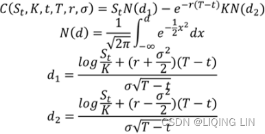
The Black-Scholes model helps determine the fair price of an option with the assumption that
- the returns of the underlying security are normally distributed (N(.))
- or that asset prices are log-normally distributed.
The formula takes on the following assumed variables—
- the strike price (K),
- the time to expiry (T),
- the risk-free rate (r),
- the volatility of the underlying returns (σ),
- the current price of the underlying asset (S),
- and its yield (q) : the dividend yield.
The mathematical formula for a call option, C(S,t), is represented as follows:![]()
Here:
By way of market forces, the price of an option may deviate(/ˈdiːvieɪt/ 偏离) from the price that's been derived from the Black-Scholes formula. In particular, the realized volatility已实现的波动率 (that is, the observed volatility of the underlying returns from historical market prices) could differ from the volatility value as implied by the Black-Scholes model, which is indicated by σ.
Think back to the Capital Asset Pricing Model (CAPM) discussed in Chapter 2https://blog.csdn.net/Linli522362242/article/details/125546725 , The Importance of Linearity in Finance. In general, securities that have higher returns exhibit higher risk, as indicated by the volatility or standard deviation of returns.
With volatility being such an important factor in security pricing, many volatility models have been proposed for studies. One such model is the implied volatility modeling of option prices.
Suppose we plot the implied volatility values of an equity option given by the Black-Scholes formula with a particular maturity for every strike price available. In general, we get a curve commonly known as the volatility smile due to its shape:
##################################################################
the binomial distribution
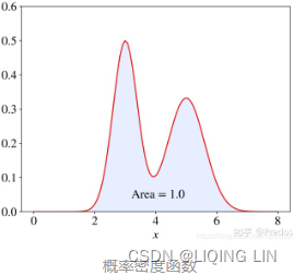
- 概率密度函数(Probability Density Function, PDF, 连续性数据)

where n is the number of trials, p is the probability of success, and N is the number of successes.
- 概率质量函数(Probability Mass Function, PMF,离散型数据)


 是离散随机变量在各特定取值上的概率
 - 概率质量函数PMF是对离散 随机变量定义的,本⾝代表该值的概率;
- 概率密度函数PDF是对连续 随机变量定义的,本⾝不是概率,只有对连续 随机变量的概率密度函数PDF在某区间内进⾏积分后才是概率
- The cumulative distribution function (cdf) or distribution function of a random variable X of the continuous type, defined in terms of the pdf of X, is given by
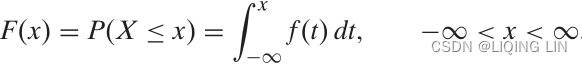
Here, again, F(x) accumulates (or, more simply, cumulates) all of the probability less
than or equal to x. From the fundamental theorem of calculus, we have, for x values
for which the derivative exists,
  = f(x)=f(k) and we call f(x) the probability
density function (pdf) of X.
In financial mathematics, the implied volatility(IV) of an option constract is the value of volatility of the underlying instrument which, when input is an option pricing model (such as Black-Scholes) will return a theoretical value equal to the current market price of the option.
##############
If X is N(μ,![]() ), then Z = (X − μ)/σ is N(0,1).
), then Z = (X − μ)/σ is N(0,1). 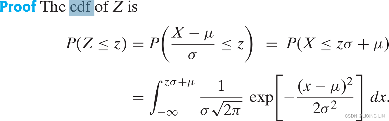
Now, for the integral积分 representing P(Z ≤ z), we use the change of variable of integration given by w = (x − μ)/σ (i.e., x = wσ + μ ==> dx = σdw ) to obtain 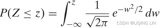
But this is the expression for ![]() , the cdf of a standardized normal random variable. Hence, Z is N(0,1).
, the cdf of a standardized normal random variable. Hence, Z is N(0,1).
help(stats.norm.cdf)Help on method cdf in module scipy.stats._distn_infrastructure:
cdf(x, *args, **kwds) method of scipy.stats._continuous_distns.norm_gen instance
Cumulative distribution function of the given RV.
Parameters
----------
x : array_like
quantiles
arg1, arg2, arg3,... : array_like
The shape parameter(s) for the distribution (see docstring of the
instance object for more information)
loc : array_like, optional
location parameter (default=0)
scale : array_like, optional
scale parameter (default=1)
Returns
-------
cdf : ndarray
Cumulative distribution function evaluated at `x`
The probability density function for norm is: for a real number x.
The probability density above is defined in the “standardized” form. To shift and/or scale the distribution use the loc and scale parameters. Specifically, norm.pdf(x, loc, scale) is identically equivalent to norm.pdf(y)/scale with y=(x-loc)/scale. Note that shifting the location of a distribution does not make it a “noncentral” distribution; noncentral generalizations of some distributions are available in separate classes.
Implied volatility#################################
![]() when t=0, the dividend yield q=0,
when t=0, the dividend yield q=0,
==>
The Black-Scholes-Merton option model is a closed-form solution to price a European option on a stock which does not pay any dividends(q=0) before its maturity date(T). If we use
 or the price today(t=0),
- K or X for the exercise price,
- r for the continuously compounded risk-free rate,
- T for the maturity in years,
- σ for the volatility of the stock
the closed-form formulae for a European call (c) and put (p) are:
- # S==S0 as t==0 K==X initial
- def black_scholes_merton(S, r, sigma, X,T):
- S = float(S) #convert to float
-
- d1 =( log(S/X) + ( (r + 0.5* sigma**2)*T) ) / ( sigma*sqrt(T) )
- # d2 =( log(S/X) + ( (r - 0.5* sigma**2)*T) ) / ( sigma*sqrt(T) )
- d2 = d1 - sigma * sqrt(T)
-
- # call option
- # stats.norm.cdf -> cumulative distribution function X~N(0,1)=N(u,sigma**2)
- # u sigma square - variance
- value = ( S * stats.norm.cdf(d1, 0.0, 1.0) -
- X * exp(-r * T) * stats.norm.cdf(d2, 0.0, 1.0))
-
- return value # present value of the European call option
In particular, the realized volatility已实现的波动率 (that is, the observed volatility of the underlying returns from historical market prices) could differ from the volatility value as implied by the Black-Scholes model, which is indicated by σ. 

the derivative of F(x)= = f(x)=f(k) and we call f(x) the probability density function (pdf) of X.
- # the partial derivative of the option pricing formula
- # with respect to to the volatility is called Vega
- def vega(S, r, sigma, X, T):
- S = float(S)
-
- d1 =( log(S/X) + ( (r + 0.5* sigma**2)*T) ) / ( sigma*sqrt(T) )
-
- vagaValue = S * stats.norm.pdf(d1, 0.0, 1.0) * sqrt(T)
-
- return vagaValue
-
- # sigma_est: initial Val # it : iteration=100
- # X: strike price or exercise prices
- # T: time to expiration
- # Cstar: the quoted price of the call option is given
- def impliedVolatility(S, r, sigma_est, X, T, Cstar, it):#######################
-
- for i in range(it):
- numer = black_scholes_merton(S, r, sigma_est, X, T) - Cstar
- denom = vega(S,r,sigma_est, X, T)
- sigma_est -= numer/denom
-
- return sigma_est #sigma_estimated #implied volatilty

!pip install tables
- from math import log, sqrt, exp
- from scipy import stats
- import pandas as pd
- import matplotlib.pyplot as plt
-
- colors = [(31, 119, 180), (174, 199, 232), (255,128,0),
- (255, 15, 14), (44, 160, 44), (152, 223, 138), (214, 39, 40),
- (255, 152, 150),(148, 103, 189), (197, 176, 213), (140, 86, 75),
- (196, 156, 148),(227, 119, 194), (247, 182, 210), (127, 127, 127),
- (199, 199, 199),(188, 189, 34), (219, 219, 141), (23, 190, 207),
- (158, 218, 229)]
- # Scale the RGB values to the [0, 1] range,
- # which is the format matplotlib accepts.
- for i in range(len(colors)):
- r, g, b = colors[i]
- colors[i] = (r / 255., g / 255., b / 255.)
- # S==S0 as t==0 K==X initial
- def black_scholes_merton(S, r, sigma, X,T):
- S = float(S) #convert to float
-
- d1 =( log(S/X) + ( (r + 0.5* sigma**2)*T) ) / ( sigma*sqrt(T) )
- # d2 =( log(S/X) + ( (r - 0.5* sigma**2)*T) ) / ( sigma*sqrt(T) )
- d2 = d1 - sigma * sqrt(T)
-
- # call option
- # stats.norm.cdf -> cumulative distribution function X~N(0,1)=N(u,sigma**2)
- # u sigma square - variance
- value = ( S * stats.norm.cdf(d1, 0.0, 1.0) -
- X * exp(-r * T) * stats.norm.cdf(d2, 0.0, 1.0))
-
- return value # present value of the European call option
-
- # the partial derivative of the option pricing formula
- # with respect to to the volatility is call Vega
- def vega(S, r, sigma, X, T):
- S = float(S)
-
- d1 =( log(S/X) + ( (r + 0.5* sigma**2)*T) ) / ( sigma*sqrt(T) )
-
- vagaValue = S * stats.norm.pdf(d1, 0.0, 1.0) * sqrt(T)
-
- return vagaValue
-
- # sigma_est: initial Val # it : iteration=100
- # X: strike price or exercise prices
- # T: time-to-maturity in year fractions
- # Cstar: the quoted price of the call option is given
- def impliedVolatility(S, r, sigma_est, X, T, Cstar, it):#######################
-
- for i in range(it):
- numer = (black_scholes_merton(S, r, sigma_est, X, T) - Cstar)
- denom = vega(S,r,sigma_est, X, T)
- sigma_est -= numer/denom
-
- return sigma_est #sigma_estimated #implied volatilty
- import pandas as pd
-
- # https://github.com/obieda01/Python-for-Finance-O-Reilly-/blob/master/ipython3/source/vstoxx_data_31032014.h5
- h5 = pd.HDFStore('vstoxx_data_31032014.h5', 'r',encoding='utf-8')
-
- futures_data = h5['futures_data'] # VSTOXX futures data
- options_data = h5['options_data'] # VSTOXX call option data
-
- h5.close()
We need the futures data to select a subset of the VSTOXX options given their (forward) moneyness. 8 futures八种期货 on the VSTOXX are traded at any time. Their maturities are the next 8 third Fridays of the month. At the end of March, there are futures with maturities ranging from the third Friday of April to the third Friday of November. TTM in the following pandas table represents time-to-maturity in year fractions以 年 分数表示的到期时间:
- futures_data['DATE']= pd.to_datetime(futures_data['DATE'])
- futures_data['MATURITY']= pd.to_datetime(futures_data['MATURITY'])
- futures_data

- options_data['DATE']= pd.to_datetime(options_data['DATE'])
- options_data['MATURITY']= pd.to_datetime(options_data['MATURITY'])
- options_data
PRICE: option market price/option quote
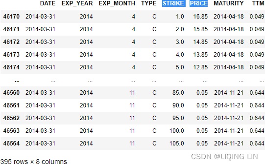
The options data set is larger since at any given trading day multiple call and put options are traded per maturity date. The maturity dates, however, are the same as for the futures. There are a total of 395 call options quoted on March 31, 2014:
options_data.info() 
As is obvious in the pandas table,
- there are call options traded and quoted that are far in-the-money (index level (PRICE) much higher than option strike (STRIKE)).
- There are also options traded that are far out-of-the-money (index level (PRICE) much lower than option strike(STRIKE)).
We therefore want to restrict the analysis to those call options with a certain (forward) moneyness货币性, given the value of the future for the respective maturity. We allow a maximum deviation of 50% from the futures level(PRICE) : tol = 0.5 .
- futureVal = futures_data[ futures_data['MATURITY'] ==\
- options_data.loc[option]['MATURITY']
- ]['PRICE'].values[0]
-
- futureVal * (1-tol) < options_data.loc[option]['STRIKE'] < futureVal * (1+tol)
Before we can start, we need to define a new column['IMP_VOL'] in the options_data DataFrame object to store the results.
- options_data['IMP_VOL'] = 0.0 # initial implied volatility####
-
- # (we change from S0 to V0 to indicate that
- # we are now working with the volatility index)
- V0 = 17.6639 # the closing value of the index
- r=0.04 # risk free interest rate
- sigma_est = 2
-
- # maximum deviation of 50% from the futures level(PRICE)
- tol = 0.5 # tolerance level for moneyness
The following code now calculates the implied volatilities for all those call options:
- for option in options_data.index:
- # iterating over all option quotes or quoted price
- futureVal = futures_data[ futures_data['MATURITY'] ==\
- options_data.loc[option]['MATURITY']
- ]['PRICE'].values[0]
-
- # picking the right futures values
- if( futureVal * (1-tol) < options_data.loc[option]['STRIKE'] < futureVal * (1+tol) ):
- # impliedVolatility(S, r, sigma_est, X, T, Cstar, it):
- # TTM or T : time-to-maturity in year fractions
- impliedVol = impliedVolatility(V0,
- r, # short rate
- sigma_est, #volatility inital value or first
- options_data.loc[option]['STRIKE'],
- options_data.loc[option]['TTM'],
- options_data.loc[option]['PRICE'], #option market price/option quote
- it=100)#iterations
- options_data['IMP_VOL'].loc[option] = impliedVol################################
-
- options_data.loc[46170]

OR
- for option in options_data.index:
- # iterating over all option quotes or quoted price
- futureVal = futures_data[ futures_data['MATURITY'] ==\
- options_data.loc[option,'MATURITY']
- ]['PRICE'].values[0]
-
- # picking the right futures values
- if( futureVal * (1-tol) < options_data.loc[option,'STRIKE'] < futureVal * (1+tol) ):
- # impliedVolatility(S, r, sigma_est, X, T, Cstar, it):
- # TTM or T : time-to-maturity in year fractions
- impliedVol = impliedVolatility(V0,
- r, # short rate
- sigma_est, #volatility inital value or first
- options_data.loc[option,'STRIKE'],
- options_data.loc[option,'TTM'],
- options_data.loc[option,'PRICE'], #option market price/option quote
- it=100)#iterations
- options_data['IMP_VOL'].loc[option] = impliedVol################################
-
- options_data.loc[46170]

The implied volatilities for the selected options shall now be visualized. To this end, we use only the subset of the options_data object for which we have calculated the implied volatilities:
- plot_data = options_data[ options_data['IMP_VOL']>0 ]#
- plot_data

To visualize the data, we iterate over all maturities of the data set and plot the implied volatilities both as lines and as single points. Since all maturities appear multiple times, we need to use a little trick to get to a nonredundent, sorted list with the maturities. The set() operation gets rid of all duplicates, but might deliver an unsorted set of the maturities. Therefore, we sort the set object
- from datetime import datetime
-
- maturities = sorted( set(options_data['MATURITY']) )
- maturities

The following code iterates over all maturities and does the plotting. The result is shown as Figure 3-1. As in stock or foreign exchange markets, you will notice the so-called volatility smile, which is most pronounced for the shortest maturity(for example: maturity.date()== 2014-04-18)在期限最短的情况下最为明显 and which becomes a bit less pronounced for the longer maturities:
- #plot_data = options_data[ options_data['IMP_VOL']>0 ]
- #maturities = sorted( set(options_data['MATURITY']) )
-
- plt.figure(figsize =(15,10))
-
- i=0
- for maturity in maturities:
- data = plot_data.loc[ options_data.MATURITY == maturity ]
-
- # select data for this maturity
- plot_args = {'lw':3, 'markersize': 9}
- plt.plot( data['STRIKE'], data['IMP_VOL'],
- label=maturity.date(),
- marker='o', color=colors[i], **plot_args
- )
- i+=1
-
- plt.grid(True)
- plt.xlabel( r'Strike Price $X$', fontsize=18 )
- plt.ylabel( r'Implied volatility of $\sigma$', fontsize=18 )
- plt.title( 'Short Maturity Window (Volatility Smile)', fontsize=22 )
-
- plt.legend()
- plt.show()

The option quotes for the day March 31, 2014 are uniquely described (“identified”) by a combination of the maturity and the strike — i.e., there is only one call option per maturity and strike.
#################################
##################################################################
The Implied volatility typically is at its highest for deep in-the-money( Call options are “in the money” when the stock price is above the strike price at expiration) and out-of-the-money options深度价内和价外期权的隐含波动率通常最高 driven by heavy speculation(/ˌspekjuˈleɪʃn/投机) and at its lowest for at-the-money options价内期权的隐含波动率最低.
The characteristics of options are explained as follows:
- In-the-money options (ITM):
- A call option is considered ITM when its strike price is below the market price of the underlying asset.
- A put option is considered ITM when its strike price is above the market price of the underlying asset.
- ITM options have an intrinsic value when exercised.ITM 期权在行使时具有内在价值
- Out-of-the-money options (OTM):
- A call option is considered OTM when its strike price is above the market price of the underlying asset.
- A put option is considered OTM when its strike price is below the market price of the underlying asset.
- OTM options have no intrinsic value when exercised, but may still have time value.
- At-the-money options (ATM):
- An option is considered ATM when its strike price is the same as the market price of the underlying asset.
- ATM options have no intrinsic value, but may still have time value.
From the preceding volatility curve, one of the objectives in implied volatility modeling is to
- seek the lowest implied volatility value possible or, in other words, to find the root.
- When found,
- the theoretical price of an ATM option(At-the-money options) for a particular maturity can be deduced被推断
- and compared against the market prices for potential opportunities, such as for studying near ATM options or far OTM(Out-of-the-money options) options.
However, since the curve is nonlinear, linear algebra cannot adequately solve the root. We will take a look at a number of root-finding methods in the next section, Root-finding algorithms.
The Markov regime-switching model马尔可夫区制转移模型
To model nonlinear behavior in economic and financial time series, Markov switching models can be used to characterize time series in different states of the world or regimes. Examples of such states could be a volatile(/ˈvɑːlətl/易变的,动荡不定的,反复无常的) state, as seen in the 2008 global economic downturn, or the growth state of a steadily recovering economy. The ability to transition转换 between these structures lets the model capture complex dynamic patterns.
The Markov property of stock prices implies that only the present values are relevant for predicting the future. Past stock-price movements are irrelevant to the way the present has emerged.(In general, however, stochastic processes used in finance exhibit the Markov property, which mainly says that tomorrow’s value of the process only depends on today’s state of the process, and not any other more “historic” state or even the whole path history. The process then is also called memoryless)
Let's take an example of a Markov regime-switching model with m=2 regimes:
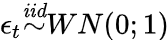
![]() ϵt is an independent and identically-distributed (i.i.d) white noise. White noise is a normally-distributed random process with a mean of zero. The same model can be represented with dummy variables:
ϵt is an independent and identically-distributed (i.i.d) white noise. White noise is a normally-distributed random process with a mean of zero. The same model can be represented with dummy variables:
The application of Markov switching models includes representing the real GDP growth rate and inflation rate dynamics. These models in turn drive the valuation models of interest-rate derivatives. The probability of switching from the previous state, i, to the current state, j, can be written as follows:![]()
#############################
n05_Reinforcement Q-Learnining_MDP_getattr_Monte Carlo_Blackjack_Driving office_ε-greedy_SARSA_Bellm_LIQING LIN的博客-CSDN博客

Central idea of MDP: MDP works on the simple Markovian property of a state; for example,  is entirely dependent on latest state
  rather than any historic dependencies. In the following equation, the current state captures all the relevant information from the history, which means the current state is a sufficient statistic of the future:
![]() ==>
==> 
#############################
The threshold autoregressive model
One popular class of nonlinear time series models is the threshold autoregressive (TAR) model, which looks very similar to the Markov switching models. Using regression methods, simple AR models are arguably(/ ˈɑːrɡjuəbli /可论证地,按理, 可以认为地) the most popular models to explain nonlinear behavior. Regimes(OR states) in the threshold model are determined by past, d, values of its own time series, relative to a threshold value, c.
The Threshold Autoregression (TAR) model is an autoregression allowing for two or more branches governed by the values for a threshold variable![]() . This allows for asymmetric behavior that can’t be explained by a single ARMA model. For a two branch model, one way to write this is:
. This allows for asymmetric behavior that can’t be explained by a single ARMA model. For a two branch model, one way to write this is:
A SETAR model (Self-Exciting TAR) is a special case where the threshold variable is y itself.
The following is an example of a self-exciting TAR (SETAR) model. The SETAR model is self-exciting because switching between different regimes depends on the past values d of its own time series:
AR(1): ![]()
 the threshold variable is
 ![]()
Using dummy variables, the SETAR model can also be represented as follows: 
The use of the TAR(threshold autoregressive) model may result in sharp transitions急剧转换 between the states as controlled by the threshold variable, c.
#################################################################
Backshift notation
The backward shift operator BB is a useful notational device when working with time series lags:![]()
Some references use L for “lag” instead of B for “backshift”.) In other words, B, operating on ![]() , has the effect of shifting the data back one period. Two applications of B to
, has the effect of shifting the data back one period. Two applications of B to![]() shifts the data back 2 periods:
shifts the data back 2 periods:![]()
For monthly data, if we wish to consider “the same month last year,” the notation is ![]() =
= ![]() .
.
The backward shift operator is convenient for describing the process of differencing差分
(
The differenced series is the change between consecutive observations in the original series, and can be written as![]() The differenced series will have only T−1 values, since it is not possible to calculate a difference
The differenced series will have only T−1 values, since it is not possible to calculate a difference ![]() for the first observation
for the first observation
). A 1st difference can be written as ![]()
Note that a first difference is represented by (1−B). Similarly, if 2nd-order differences have to be computed, then:
![]()
In general, a dth-order difference can be written as ![]()
Backshift notation is particularly useful when combining differences, as the operator can be treated using ordinary algebraic rules. In particular, terms involving B can be multiplied together.
For example, a seasonal difference followed by a first difference![]() (where m= the number of seasons. These are also called “lag-m differences”, as we subtract the observation after a lag of m periods.
(where m= the number of seasons. These are also called “lag-m differences”, as we subtract the observation after a lag of m periods.
then the twice-differenced series is ) can be written as
 the same result we obtained earlier.
When the differenced series is white noise, the model for the original series can be written as ![]()
where![]() denotes white noise. Rearranging this leads to the “random walk” model
denotes white noise. Rearranging this leads to the “random walk” model ![]()
Random walk models are widely used for non-stationary data, particularly financial and economic data. Random walks typically have:
- long periods of apparent trends up or down
- sudden and unpredictable changes in direction.
A closely related model allows the differences to have a non-zero mean. Then ![]()
The value of c is the average of the changes between consecutive observations.
- If c is positive, then the average change is an increase in the value of
 . Thus, will tend to drift upwards.
 - However, if c is negative, will tend to drift downwards.
autoregressive (AR) mode
The notation AR(p) indicates an autoregressive model of order p (p阶). The AR(p) model is defined as![]() OR
OR![]()
where are the parameters of the model, c is a constant, and
  is white noise(lagged value, White noise is a normally-distributed random process with a mean of 0). This can be equivalently written using the backshift operator B后移运算符 as

so that, moving the summation term to the left side and using polynomial notation, we have
![]()

![]() We refer to this as an AR(p) model, an autoregressive model of order pp.
We refer to this as an AR(p) model, an autoregressive model of order pp.
AR(1) : AR(P=1)==>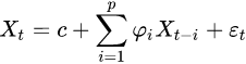 ==>
==>![]()
- when
 =0, (or
  ) is equivalent to white noise;
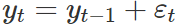
 - when ϕ1=1 and c=0, (or ) is equivalent to a random walk;
- when ϕ1=1 and c≠0, is equivalent to a random walk with drift;

The value of c is the average of the changes between consecutive observations - when ϕ1<0, (or ) tends to oscillate around the mean.
We normally restrict autoregressive models to stationary data, in which case some constraints on the values of the parameters are required.
- For an AR(1) model: −1<<1.
- For an AR(2) model: −1<<1, ϕ1+ϕ2<1, ϕ2−ϕ1<1.
When p≥3, the restrictions are much more complicated.
Some parameter constraints are necessary for the model to remain wide-sense stationary保持广义平稳. For example, processes in the AR(1) model with![]() are not stationary. More generally, for an AR(p) model to be wide-sense stationary, the roots of the polynomial
are not stationary. More generally, for an AR(p) model to be wide-sense stationary, the roots of the polynomial ![]() OR
OR must lie outside the unit circle
 , i.e., each (complex) root
 ![]() must satisfy
must satisfy ![]() .
.
Intertemporal effect of shocks冲击的跨期效应
AR(1) : AR(P=1)==> ==>![]()
In an AR process, a one-time shock affects values of the evolving variable infinitely far into the future. For example, consider the AR(1) model . A non-zero value for 
- at say time t=1 affects
 by the amount
  .
. - Then by the AR equation for
 in terms of , this affects by the amount
  .
. - Then by the AR equation for
 in terms of , this affects by the amount
  .
. - Continuing this process shows that the effect of never ends, although if the process is stationary then the effect diminishes(/ dɪˈmɪnɪʃt /减少,削弱) toward 0 in the limit.
Because each shock affects X values infinitely far into the future from when they occur, any given value ![]() is affected by shocks occurring infinitely far into the past. This can also be seen by rewriting the autoregression
is affected by shocks occurring infinitely far into the past. This can also be seen by rewriting the autoregression![]() <==
<==![]()
![]() ( where the constant term c has been suppressed常数项已被抑制 by assuming that the variable
( where the constant term c has been suppressed常数项已被抑制 by assuming that the variable![]() has been measured as deviations from its mean) as
has been measured as deviations from its mean) as 
When the polynomial division on the right side is carried out, the polynomial in the backshift operator B后移运算符 applied to has an infinite order无限阶—that is, an infinite number of lagged values滞后值 of appear on the right side of the equation.
OR![]()

![]() OR(where the constant term c has been suppressed常数项已被抑制 by assuming that the variable has been measured as deviations from its mean) ==> backshift operator B后移运算符
OR(where the constant term c has been suppressed常数项已被抑制 by assuming that the variable has been measured as deviations from its mean) ==> backshift operator B后移运算符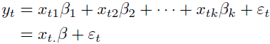
A simple AR(1) model is ![]() ==>
==>![]() ==>Subtract
==>Subtract ![]() from both sides==>
from both sides==>![]()
where
 is the variable of interest,
- t is the time index,
 is a coefficient(or w or θ or
  ),
),
- if -1<<1, the model would be stationary
- ==1, the series is non-stationary,


- >1,
 , the series is divergent and the difference series is non-stationary
 - Therefore, judging whether a sequence is stable can be achieved by checking whether is strictly less than 1.
- if -1<
 is the error term (assumed to be white noise or lagged value).
- A unit root is present if =1. The model would be non-stationary in this case.
The regression model(OLS) can be written as
where is the first difference operator and
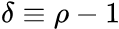 . This model can be estimated and testing for a unit root is equivalent to testing
  . Since the test is done over the residual term rather than raw data, it is not possible to use standard t-distribution to provide critical values. Therefore, this statistic t has a specific distribution simply known as the Dickey–Fuller table.==>


There are three main versions of the test:
- 1. Test for a unit root:

- 2. Test for a unit root with constant
 :
: 
- 3. Test for a unit root with constant and deterministic time trend:

Each version of the test has its own critical value临界值 which depends on the size of the sample. In each case, the null hypothesis is that there is a unit root, . The tests have low statistical power in that they often cannot distinguish between true unit-root processes () and near unit-root processes (
  is close to zero). This is called the "near observation equivalence"近观测等效 problem.
vvvvvvvvvvvvvvvvvvvvvvvvvvvvvvstatistical powerhttps://blog.csdn.net/Linli522362242/article/details/121721868
 vs
vs 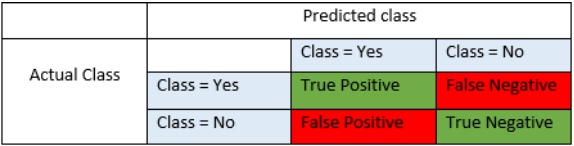

- T: True prediction or classify correctly; F: False prediction or classify incorrectly
P: instance is truely belong to target class(the null hypothesis=False, Reject,when a specific alternative hypothesis ( ) is true) based on the fact;
N: instance is not belong to target class(the null hypothesis=True, Accept ) based on the fact - Type I error(FP): Rejecting a null hypothesiswhen it is true, (OR is true, but we reject it by mistake. Because we mistakenly think is False, ###wrongly reject
P=target class(the null hypothesis=False, Reject) )
- α = probability of a Type I error, known as a "false positive"(FP), is actually true, but we reject it by mistake since we mistakenly think is False, and mistakenly accept
- 1-α = probability of a "true negative"(TN), i.e., correctly not rejecting the null hypothesis, since =True, non-false ### correctly accept and correctly reject
- α = probability of a Type I error, known as a "false positive"(FP),
- Type II error(FN): Accepting a null hypothesiswhen it is false, (OR is false, but we fail to reject it.)
- β = probability of a Type II error, known as a "false negative"(FN) ( Because we mistakenly think is True, N=non-target class(the null hypothesis=True, Accept)) ### wrongly failing错误地没有 to reject it
- 1-β = probability of a "true positive"(TP), i.e., correctly rejecting the null since=False, when a specific alternative hypothesis () is true.
- β = probability of a Type II error, known as a "false negative"(FN) ( Because we mistakenly think
The statistical power of a binary hypothesis test is the probability that the test correctly rejects the null hypothesis (![]() ) when a specific alternative hypothesis (
) when a specific alternative hypothesis (![]() ) is true(since
) is true(since![]() =False, reject
=False, reject![]() ). It is commonly denoted by
). It is commonly denoted by ![]() (1-β = probability of a "true positive"(TP), i.e., correctly rejecting the null
(1-β = probability of a "true positive"(TP), i.e., correctly rejecting the null![]() since
since![]() =False), and represents the chances of a "true positive"(TP) detection conditional on the actual existence of an effect to detect. Statistical power ranges from 0 to 1, and as the power of a test increases(1-β), the probability
=False), and represents the chances of a "true positive"(TP) detection conditional on the actual existence of an effect to detect. Statistical power ranges from 0 to 1, and as the power of a test increases(1-β), the probability![]() of making a type II error by wrongly failing to reject the null hypothesis decreases.
of making a type II error by wrongly failing to reject the null hypothesis decreases.
β = probability of a Type II error, known as a "false negative"(FN) ( Because we mistakenly think ![]() is True, N=non-target class(the null hypothesis
is True, N=non-target class(the null hypothesis![]() =True, Accept
=True, Accept![]() ))
))
To measure the likelihood of making Type I or II error, we define: 
- α = probability of a Type I error, known as a "false positive"(FP), is actually true, but we reject it by mistake since we mistakenly think is False, and mistakenly accept
- β = probability of a Type II error, known as a "false negative"(FN) ( Because we mistakenly think is True, N=non-target class(the null hypothesis=True, Accept), wrongly failing错误地没有 to reject the null hypothesis (wrongly accept ) but wrongly reject )
Statistical power ranges from 0 to 1, and as the power of a test increases(1-β), the probability of making a type II error by wrongly failing to reject the null hypothesis decreases.
Ideally, we want both α and to β be small. However, if we decrease α, we increase β, and vice-versa.
A Type I error is when we reject a true null hypothesis (FP: ![]() is actually true, but we reject it by mistake since we mistakenly think
is actually true, but we reject it by mistake since we mistakenly think ![]() is False, and mistakenly accept
is False, and mistakenly accept ![]() ).
).
Lower values of α
(
α=the probability of a Type I error=the probability of FP : mistakenly think ![]() is False and then reject
is False and then reject ![]() , so choosing lower values for α can reduce the probability of a Type I error.
, so choosing lower values for α can reduce the probability of a Type I error.
)
make it harder to reject the null hypothesis![]()
<
larger 1-α ==> larger TN == increase the probility of correctly accept true null hypothesis![]() ==> lower the probility to reject a true null hypothesis
==> lower the probility to reject a true null hypothesis![]() and we prefer to accept the null hypothesis as true:
and we prefer to accept the null hypothesis as true:![]() =True
=True
>,
The consequence here is that if the null hypothesis![]() is actually false, it may be more difficult to reject using a low value for α
is actually false, it may be more difficult to reject using a low value for α
(since we prefer to accept the null hypothesis as true).
So using lower values of α can increase the probability of a Type II error (FN : Because we mistakenly think ![]() is True, N=non-target class(the null hypothesis
is True, N=non-target class(the null hypothesis![]() =True, Accept
=True, Accept![]() )), increase β.
)), increase β.
A Type II error( FN : Because we mistakenly think ![]() is True, N=non-target class(the null hypothesis
is True, N=non-target class(the null hypothesis![]() =True, Accept
=True, Accept![]() )) is when we fail to reject a false null hypothesis
)) is when we fail to reject a false null hypothesis![]() . Higher values of α ( α=the probability of a Type I error=the probability of FP : mistakenly think
. Higher values of α ( α=the probability of a Type I error=the probability of FP : mistakenly think ![]() is False and then reject
is False and then reject ![]() ) make it easier to reject the null hypothesis
) make it easier to reject the null hypothesis![]() , so choosing higher values for α can reduce the probability of a Type II error(since we prefer to believe the null hypothesis
, so choosing higher values for α can reduce the probability of a Type II error(since we prefer to believe the null hypothesis ![]() =False). The consequence here is that if the null hypothesis
=False). The consequence here is that if the null hypothesis![]() is true, increasing α makes it more likely that we commit a Type I error (rejecting a true null hypothesis).
is true, increasing α makes it more likely that we commit a Type I error (rejecting a true null hypothesis).
Summary:
We will make α small(increase 1-α, TN, we prefer to accept the null hypothesis as true):
If we want reject ![]() , we need to be pretty sure it's false
, we need to be pretty sure it's false
we will fail to reject没有拒绝 False null hypothesis , we believe is true because we may have a big chance(large β) to make Type II error when
 ![]() is actually False based on the fact.
is actually False based on the fact.
Example 1
Employees at a health club do a daily water quality test in the club's swimming pool. If the level of contaminants(/ kənˈtæmɪnənt /污染物) are too high, then they temporarily close the pool to perform a water treatment.
We can state the hypotheses for their test as: The water quality is acceptable vs. ![]() : The water quality is not acceptable.
: The water quality is not acceptable.
What would be the consequence of a Type I error(FP) in this setting?
A Type I error is when we reject a true ![]() . In this setting, if
. In this setting, if ![]() is true, then the water quality is acceptable, and the pool doesn't need to be closed. A Type I error would occur if they close the pool when it doesn't need to be closed since the water quality is actually acceptable.
is true, then the water quality is acceptable, and the pool doesn't need to be closed. A Type I error would occur if they close the pool when it doesn't need to be closed since the water quality is actually acceptable.
What would be the consequence of a Type II error(FN) in this setting?
A Type II error is when we fail to reject a false ![]() . In this setting, if
. In this setting, if ![]() is false, then the water quality is not acceptable, and the pool should be closed. A Type II error would occur if they don't close the pool when it needs to be closed since the water quality is not actually acceptable.
is false, then the water quality is not acceptable, and the pool should be closed. A Type II error would occur if they don't close the pool when it needs to be closed since the water quality is not actually acceptable.
In terms of safety, which error has the more dangerous consequences in this setting?
Type II error
The consequence here is that people swim in contaminated water. This is more dangerous than a Type I error.
Since one error involves greater safety concerns, the club is considering using a value for α other than 0.05 for the water quality significance test.由于一个错误涉及更大的安全问题,俱乐部正在考虑使用 0.05 以外的 α 值进行水质显着性检验
What significance level should they use to reduce the probability of the more dangerous error?
Higher α ==>prefer to reject a true![]() since we prefer to belive
since we prefer to belive ![]() =False(
=False(![]() :The water quality is not acceptable)
:The water quality is not acceptable)
Lower α ==>harder to reject the null hypothesis true![]() since we prefer to belive
since we prefer to belive ![]() =True(
=True(![]() :The water quality is acceptable),
:The water quality is acceptable),
Using a higher significance level (α=0.10 > 0.05) increases the probability of a Type I error, but decreases the probability of a Type II error (which is more dangerous in this setting).
Example 2
Seth is starting his own food truck business, and he's choosing cities where he'll run his business. He wants to survey residents and test whether or not the demand is high enough to support his business before he applies for the necessary permits to operate in a given city. He'll only choose a city if there's strong evidence that the demand there is high enough.
We can state the hypotheses for his test as ![]() : The demand is not high enough vs.
: The demand is not high enough vs. ![]() :The demand is high enough.
:The demand is high enough.
What would be the consequence of a Type I error(FP) in this setting?
A Type I error is when we reject a true ![]() . In this setting, if
. In this setting, if ![]() is true, then demand in the city is not high enough, and Seth shouldn't choose that city. A Type I error would occur if he chooses a city where the demand is not actually high enough.
is true, then demand in the city is not high enough, and Seth shouldn't choose that city. A Type I error would occur if he chooses a city where the demand is not actually high enough.
What would be the consequence of a Type II error(FN) in this setting?
A Type II error is when we fail to reject a false ![]() . In this setting, if
. In this setting, if ![]() is false, then demand in the city is high enough, and Seth should choose that city. A Type II error would occur if he doesn't choose a city where the demand is actually high enough.
is false, then demand in the city is high enough, and Seth should choose that city. A Type II error would occur if he doesn't choose a city where the demand is actually high enough.
Seth has determined that a Type I error is more costly to his business than a Type II error. He wants to use a significance level other than α=0.05 to reduce the likelihood of a Type I error.
Higher α ==>prefer to reject a true![]() since we prefer to belive
since we prefer to belive ![]() =False(
=False(![]() :The demand is high enough.)
:The demand is high enough.)
Lower α ==>harder to reject the null hypothes is true![]() since we prefer to belive
since we prefer to belive ![]() =True(
=True(![]() : The demand is not high enough),
: The demand is not high enough),
Using a lower significance level decreases the probability of a Type I error, since it makes it more difficult to reject ![]() based on
based on ![]() =True.
=True.
#################################################################
Smooth transition models
Consider a simple AR(p) model for a time series 
![]()
where:
-
 for i=1,2,...,p are autoregressive coefficients, assumed to be constant over time;
  stands for white-noise error term with constant variance.
Variance is a measure of dispersion, meaning it is a measure of how far a set of numbers is spread out from their average value.
written in a following vector form:![]() and
and ![]() =1
=1
where:
 is a column vector of variables;
 gamma is the vector of parameters :
 ;
; stands for white-noise error term with constant variance.
Defined in this way, STAR(Smooth Transition Autoregressive) model can be presented as follows:![]()
here:
 is a column vector of variables;
 is the transition function bounded between 0 and 1.
- The models can be thought of in terms of extension of autoregressive models discussed above, allowing for changes in the model parameters according to the value of a transition variable

Basic Structure
They can be understood as two-regime SETAR model with smooth transition between regimes, or as continuum of regimes. In both cases the presence of the transition function is the defining feature of the model as it allows for changes in values of the parameters
Transition Function
Three basic transition functions and the name of resulting models are:
- first order logistic function - results in Logistic STAR (LSTAR) model:

- exponential function - results in Exponential STAR (ESTAR) model:

- second order logistic function:

Abrupt(/ əˈbrʌpt /突然的) regime changes in the threshold models appear to be unrealistic against real-world dynamics. This problem can be overcome by introducing a smoothly-changing continuous function from one regime to another. The SETAR(Self-Exciting Threshold AutoRegressive) model becomes a logistic smooth transition threshold autoregressive (LSTAR) model with the logistic function of ![]() :
: 
- The
 or
or  parameter controls the smooth transition from one regime to another.
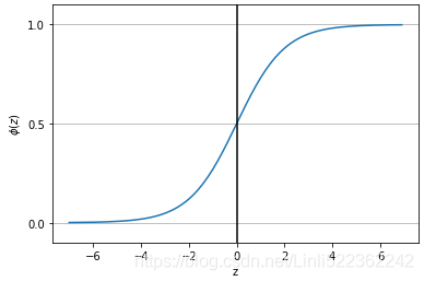
 approaches 1 if z goes towards infinity (z
  ),approaches 0 if z goes towards negative infinity ( -
 ),
), - For large values of , the transition is the fastest, as当
 approaches the threshold variable, c.
*Z= , If the smoothness parameter, , is large, the function
  becomes steep. In this case, the smooth-transition model is not distinguishable from the threshold model, because there are only two possible regimes.
 ==>*Z ==>
The SETAR(Self-Exciting Threshold AutoRegressive) model now becomes an LSTAR(logistic smooth transition threshold autoregressive) model, as shown in the following equation: ![]()
<== the threshold variable is
 ![]()
- Theor parameter controls the smooth transition from one regime to another.
- For large values of , the transition is the fastest, as当 approaches the threshold variable, c.
- When =0,==>=1 the LSTAR model is equivalent to a simple AR(1) one-regime model.

Root-finding algorithms
In the preceding section, we discussed some nonlinear models commonly used for studying economics and financial time series. From the model data given in continuous time, the intention is therefore to search for the extrema that could possibly infer valuable information. The use of numerical methods, such as root-finding algorithms, can help us find the roots of a continuous function, f, such that f(x)=0, which can either be the maxima or the minima of the function. In general, an equation may either contain a number of roots or none at all.
One example of the use of root-finding methods on nonlinear models is the Black-Scholes implied volatility modeling discussed earlier, in The implied volatility model section. An option trader would be interested in deriving implied prices based on the Black-Scholes model and comparing them with market prices. In the https://blog.csdn.net/Linli522362242/article/details/125355166, Numerical Methods for Pricing Options , we will see how we can combine a root-finding method with a numerical-option pricing procedure to create an implied volatility model based on the market prices of a particular option.
Root-finding methods use an iterative routine that requires a start point or the estimation of the root. The estimation of the root can either
- converge toward a solution,收敛到一个解
- converge to a root that is not sought,收敛到一个不被寻找的根
- or may not even find a solution at all.甚至可能根本找不到一个解
Thus, it is crucial to find a good approximation to the root.
Not every nonlinear function can be solved using root-finding methods. The following figure shows an example of a continuous function,![]() , where root-finding methods may fail to arrive at a solution. There are discontinuities at x=0 and x=2 for the y values in the range of -20 to 20:
, where root-finding methods may fail to arrive at a solution. There are discontinuities at x=0 and x=2 for the y values in the range of -20 to 20:
There is no fixed rule as to how a good approximation can be defined. It is recommended that you bracket or define the lower and upper search bounds before starting the root-finding iterative procedure. We certainly do not want to keep searching endlessly in the wrong direction for our root.
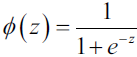
Incremental search
A crude method of solving a nonlinear function is by doing an incremental search. Using an arbitrary starting point, a, we can obtain values of f(a) for every increment of dx. We assume that the values of f(a+dx), f(a+2dx), f(a+3dx)… are going in the same direction as indicated by their sign.
- Once the sign changes, a solution is deemed as found.
- Otherwise, the iterative search terminates when it crosses the boundary point, b.
A pictorial(/ pɪkˈtɔːriəl /绘画的;形象化的) example of the root-finder method for iteration is given in the following graph:
An example can be seen from the following Python code:
- # An incremental search algorithm
-
- import numpy as np
-
- def incremental_search( func, a, b, dx ):
- """
- :param func: The function to solve
- :param a: The left boundary x-axis value
- :param b: The right boundary x-axis value
- :param dx: The incremental value in searching
- :return:
- The x-axis value of the root,
- number of iterations used
- """
-
- # f(a+dx), f(a+2dx), f(a+3dx)…
- fa = func(a)
-
- c = a + dx
- fc = func(c)
-
- n=1
- while np.sign(fa) == np.sign(fc):
- if a >= b: # the iterative search terminates when it crosses the boundary point, b.
- return a-dx, n
- a = c
- fa = fc
- c = a + dx # f(a+2dx), f(a+3dx)…
- fc = func(c)
- n += 1
-
- if fa==0: # since we start fa<0 or fc<0
- return a,n
- elif fc==0:
- return c,n
- else: # Once the sign changes, a solution is deemed as found.
- return (a+c)/2., n
At every iterative procedure, a will be replaced by c , and c will be incremented by dx before the next comparison. Should a root be found, it is plausible(/ˈplɔːzəbl/可靠的,似合理的) that it lies between a and c , both inclusive. In the event that the solution does not rest at either point, we will simply return the average of the two points as the best estimation. The n variable keeps track of the number of iterations that underwent the process of finding our root.
We will use the equation that has an analytic solution of ![]() to demonstrate and measure our root-finder, where x is bounded between -5 and 5 : [-5,5]. A small dx value of 0.001 is given, which also acts as a precision tool. Smaller values of dx produce better precision but also require more search iterations:
to demonstrate and measure our root-finder, where x is bounded between -5 and 5 : [-5,5]. A small dx value of 0.001 is given, which also acts as a precision tool. Smaller values of dx produce better precision but also require more search iterations:
- # The keyword 'lambda' creates an anonymous function
- # with input argument x
- # https://blog.csdn.net/Linli522362242/article/details/107086444
- # return x**3 + 2.*x**2 - 5
- y = lambda x: x**3 + 2.*x**2 - 5
- #[-5, 5]
- root, iterations = incremental_search( y, -5., 5., 0.001 )
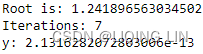
- print( "Root is:", root )
- print( "Iterations:", iterations )
- print( "y:", root**3 + 2.*root**2 - 5)

The incremental search root-finder method is a basic demonstration of the fundamental behavior of a root-finding algorithm. The accuracy is at its best when defined by dx, and consumes an extremely long computational time in the worst possible scenario. The higher the accuracy demanded, the longer it takes for the solution to converge. For practical reasons, this method is the least preferred of all root-finding algorithms, and we will take a look at alternative methods to find the roots of our equation that can give us better performance.
The bisection method
The bisection method is considered the simplest one-dimensional root-finding algorithm. The general interest is to find the value, x, of a continuous function, f, such that f(x)=0.
Suppose we know the two points of an interval, a and b, where a < b, and that f(a)<0 and f(b)>0 lie along the continuous function, taking the midpoint of this interval as c, where![]() ; the bisection method then evaluates this value as f(c).
; the bisection method then evaluates this value as f(c).
Let's illustrate the setup of points along a nonlinear function with the following graph: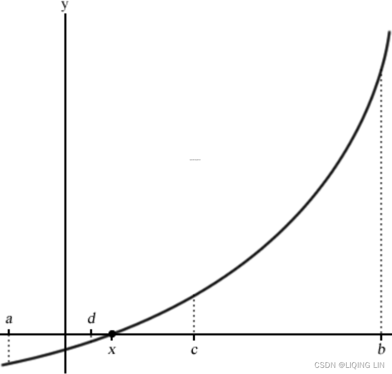

Since the value of f(a) is negative and f(b) is positive, the bisection method assumes that the root, x, lies somewhere between a and b and gives f(x)=0.
If f(c)=0 or is very close to zero by some predetermined error-tolerance value, a root is declared as found. If f(a)*f(c)<0, we may conclude that a root exists along the a and c interval, or the c and b interval otherwise.
In the next evaluation, c is replaced as either b or a accordingly. With the new interval shortened, the bisection method repeats with the same evaluation to determine the next value of c. This process continues, shrinking the width of the [a,b] interval until the root is considered found.
The biggest advantage of using the bisection method is its guarantee to converge to an approximation of the root, given a predetermined error-tolerance level and the maximum number of iterations allowed. It should be noted that the bisection method does not require knowledge of the derivative of the unknown function. In certain continuous functions, the derivative could be complex or even impossible to calculate. This makes the bisection method extremely valuable for working on functions that are not smooth.
Because the bisection method does not require derivative information from the continuous function, its major drawback is that it takes up more computational time in the iterative evaluation than other root-finder methods. Also, since the search boundary of the bisection method lies in the a and b intervals, it would require a good approximation to ensure that the root falls within this range. Otherwise, an incorrect solution may be obtained, or even none at all. Using large values of a and b might consume more computational time.
The bisection is considered to be stable without the use of an initial guess value for convergence to happen. Often, it is used in combination with other methods, such as the faster Newton's method, to converge quickly with precision.
The Python code for the bisection method is given as follows. Save this as bisection.py
- # The bisection method
- import numpy as np
-
- def bisection(func, a, b, tol=0.1, maxiter=20):
- """
- :param func: The function to solve
- :param a: The x-axis value where f(a)<0
- :param b: The x-axis value where f(b)>0
- :param tol: The precision of the solution
- :param maxiter: Maximum number of iterations
- :return:
- The x-axis value of the root,
- number of iterations used
- """
- c = (a+b)*0.5 # Declare c as the midpoint [a,b]
- n = 1 # start with 1 iteration
- while n<= maxiter:
- c = (a+b)*0.5
- # Root is found or is very close
- if func(c) == 0 or abs(a-b)*0.5 < tol:
- return c,n
- n += 1
-
- # Decide the side to repeat the steps
- if func(c) < 0:
- a=c
- else:
- b=c
-
- return c,n
https://www.geeksforgeeks.org/program-for-bisection-method/
- # The keyword 'lambda' creates an anonymous function
- # with input argument x
- # https://blog.csdn.net/Linli522362242/article/details/107086444
- # return x**3 + 2.*x**2 - 5
- y = lambda x: x**3 + 2.*x**2 - 5
- #[-5, 5]
- root, iterations = bisection( y, -5., 5., 0.00001, 100 )
- print( "Root is:", root )
- print( "Iterations:", iterations )
- print( "y:", root**3 + 2.*root**2 - 5)

Again, we bounded the anonymous lambda function to the y variable with an input parameter, x , and attempted to solve the ![]() equation as before, in the interval between -5 to 5 to an accuracy of 0.1 with a maximum iteration of 100.
equation as before, in the interval between -5 to 5 to an accuracy of 0.1 with a maximum iteration of 100.
As we can see, the result from the bisection method gives us better precision in far fewer iterations over the incremental search method.
Newton's method
![]()
Use the function ![]() to find the roots of the equation
to find the roots of the equation ![]() (i.e. all solutions to x that give
(i.e. all solutions to x that give ![]() . For example: f(x)=(x-2)(x-3), then x=2 and x=3 are both the roots of function
. For example: f(x)=(x-2)(x-3), then x=2 and x=3 are both the roots of function ![]() .
.
A graphical representation of Newton's method is shown in the following screenshot. ![]() is the initial x value. The derivative of
is the initial x value. The derivative of ![]() is evaluated, which is a tangent line crossing the x axis at
is evaluated, which is a tangent line crossing the x axis at ![]() . The iteration is repeated, evaluating the derivative at points
. The iteration is repeated, evaluating the derivative at points ![]() ,
,![]() , and so on:
, and so on:
 ==>
==>![]()
Newton's method, also known as the Newton-Raphson method, uses an iterative procedure to solve for a root using information about the derivative of a function. The derivative is treated as a linear problem to be solved. The first-order derivation, f′, of the function, f, represents the tangent line. The approximation to the next value of ![]() , given as
, given as ![]() , is as follows:
, is as follows: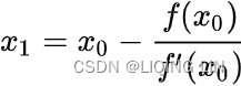 ==>
==>![]()
![]() ==>
==>![]()
Here, the tangent line intersects the x axis at ![]() , which produces y=0. This also represents the first-order Taylor expansion about
, which produces y=0. This also represents the first-order Taylor expansion about ![]() , such that that the new pont,
, such that that the new pont, ![]() , solves the following equation:
, solves the following equation: ![]()
This process is repeated with x taking the value of ![]() until the maximum number of iterations is reached, or the absolute difference between
until the maximum number of iterations is reached, or the absolute difference between ![]() and
and ![]() is within an acceptable accuracy level.
is within an acceptable accuracy level.
An initial guess value is required to compute the values of f(x) and f'(x). The rate of convergence is quadratic, which is considered to be extremely fast at obtaining the solution with high levels of accuracy.
The drawback to Newton's method is that it does not guarantee global convergence to the solution. Such a situation arises when the function contains more than one root, or when the algorithm arrives at a local extremum and is unable to compute the next step. As this method requires knowledge of the derivative of its input function, it is required that the input function be differentiable. However, in certain circumstances, it is impossible for the derivative of a function to be known, or otherwise be mathematically easy to compute.
The implementation of Newton's method in Python is as follows:
- # The Newton-Raphson method
-
- def newton(func, df, x, tol=0.001, maxiter=100):
- """
- :param func: The function to solve
- :param df: The derivative function of f
- :param x: Initial guess value of x
- :param tol: The precision of the solution
- :param maxiter: Maximum number of iterations
- :return:
- The x-axis value of the root,
- number of iterations used
- """
- n = 1
- while n<=maxiter:
- x1 = x-func(x)/df(x)
- if abs(x1-x) < tol: # the Root is very close
- return x1, n
- x = x1
- n += 1
- return None, n
We will use the same function used in the bisection example and take a look at the results from Newton's method:
- # The keyword 'lambda' creates an anonymous function
- # with input argument x
- # https://blog.csdn.net/Linli522362242/article/details/107086444
- # return x**3 + 2.*x**2 - 5
- y = lambda x: x**3 + 2.*x**2 - 5
- dy = lambda x: 3.*x**2 + 4.*x
- # x start from 5
- root, iterations = newton( y, dy, 5., 0.00001, 100 )
- print( "Root is:", root )
- print( "Iterations:", iterations )
- print( "y:", root**3 + 2.*root**2 - 5)
Beware of division by zero exceptions! In Python 2, using values such as 5.0, instead of 5, lets Python recognize the variable as a float, avoids the problem of treating variables as integers in calculations, and gives us better precision.
With Newton's method, we obtained a really close solution with less iteration over the bisection method.
The secant method割线法
The secant method uses secant lines to find the root. A secant line is a straight line that intersects two points of a curve. In the secant method, a line is drawn between two points on the continuous function, such that it extends and intersects the x axis. This method can be thought of as a Quasi-Newton method. By successively drawing such secant lines, the root of the function can be approximated.
The secant method is graphically represented in the following screenshot. An initial guess of the two x axis values, ![]() and
and ![]() , is required to find
, is required to find ![]() and
and ![]() . A secant line, y, is drawn from
. A secant line, y, is drawn from ![]() to
to ![]() and intersects at the
and intersects at the ![]() =
=![]() point on the x axis, such that:
point on the x axis, such that:
The root of this linear function, that is the value of x such that y = 0 is![]()
The solution to ![]() is therefore as follows:
is therefore as follows: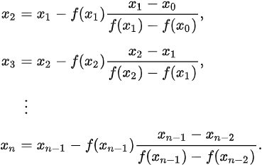
On the next iteration, ![]() and
and ![]() will take on the values of
will take on the values of ![]() and
and ![]() , respectively. The method repeats itself, drawing secant lines for the x axis values of
, respectively. The method repeats itself, drawing secant lines for the x axis values of ![]() and
and![]() ,
, ![]() and
and ![]() , and so on. The solution terminates when the maximum number of iterations has been reached, or the difference between
, and so on. The solution terminates when the maximum number of iterations has been reached, or the difference between ![]() and
and ![]() has reached a pre-specified tolerance level, as shown in the following graph:
has reached a pre-specified tolerance level, as shown in the following graph:
The rate of convergence of the secant method is considered to be superlinear. Its secant method converges much faster than the bisection method and slower than Newton's method. In Newton's method, the number of floating-point operations takes up twice as much time as the secant method in the computation of both its function and its derivative on every iteration. Since the secant method requires only the computation of its function at every step, it can be considered faster in absolute time.
The initial guess values of the secant method must be close to the root, otherwise it has no guarantee of converging to the solution.
The Python code for the secant method is given as follows:
- # The secant root-finding method
-
- def secant(func, x0, x1, tol=0.001, max_iter=100):
- """
- :param func: The function to solve
- :param a: Initial x-axis guess value
- :param b: Initial x-axis guess value, where b>a
- :param tol: The precision of the solution
- :param maxiter: Maximum number of iterations
- :return:
- The x-axis value of the root,
- number of iterations used
- """
- i = 1
- while i<= max_iter:
- x2 = x1 - func(x1) * (x1-x0)/( func(x1)-func(x0) )
-
- if abs(x2-x1) < tol:
- return x2, i
-
- x0 = x1
- x1 = x2
- i += 1
- return None, i
Again, we will reuse the same nonlinear function and return the results from the secant method:
- y = lambda x: x**3 + 2.*x**2 - 5.
- #[-5,5]
- root, iterations = secant( y, -5.0, 5.0, 0.00001, 100 )
- print( "Root is:", root )
- print( "Iterations:", iterations )
- print( "y:", root**3 + 2.*root**2 - 5)
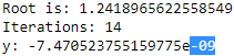
Though all of the preceding root-finding methods gave very close solutions, the secant method performs with fewer iterations compared to the bisection method,but with more than Newton's method.
The secant method converges much faster than the bisection method and slower than Newton's method. In Newton's method, the number of floating-point operations takes up twice as much time as the secant method in the computation of both its function and its derivative on every iteration. Since the secant method requires only the computation of its function at every step, it can be considered faster in absolute time.
Combing root-finding methods
It is perfectly possible to write your own root-finding algorithms using a combination of the previously-mentioned root-finding methods. For example, you may use the following implementation:
- 1. Use the faster secant method to converge the problem to a pre-specified error-tolerance value or a maximum number of iterations
- 2. Once a pre-specified tolerance level is reached, switch to using the bisection method to converge to the root by halving the search interval with each iteration until the root is found
Brent's method or the Wijngaarden-Dekker-Brent method combines the bisection root-finding method, secant method, and inverse quadratic interpolation. The algorithm attempts to use either the secant method or inverse quadratic interpolation反二次插值法 whenever possible, and uses the bisection method where necessary. Brent's method can also be found in the scipy.optimize.brentq function of SciPy.
SciPy implementations in root-finding
Before starting to write your root-finding algorithm to solve nonlinear or even linear problems, take a look at the documentation of the scipy.optimize methods. SciPy contains a collection of scientific computing functions as an extension of Python. Chances are that these open source algorithms might fit into your applications off the shelf.
Root-finding scalar functions
Some root-finding functions that can be found in the scipy.optimize modules include bisect , newton, brentq, and ridder. Let's set up the examples that we have discussed in the Incremental search section using the implementations by SciPy:
- # Documentation at
- # https://docs.scipy.org/doc/scipy/reference/optimize.html
-
- import scipy.optimize as optimize
-
- y = lambda x: x**3 + 2.*x**2 - 5.
- dy = lambda x: 3.*x**2 + 4.*x
-
- # Call method: bisect(f, a, b[, args, xtol, rtol, maxiter, ...])
- # [-5,5]
- print( "Bisection method:", optimize.bisect(y, -5, 5., xtol=0.00001) )
-
- # When fprime=None, then the secant method is used.
- # https://docs.scipy.org/doc/scipy/reference/generated/scipy.optimize.newton.html#scipy.optimize.newton
- print( "Newton's method:", optimize.newton(y, 5., fprime=dy) )
-
- # fprime : The derivative of the function #x0
- print( "Secant method:", optimize.newton(y, 5.) )
-
- # Call method: brentq(f, a, b[, args, xtol, rtol, maxiter, ...])
- print( "Brent's method:", optimize.brentq(y, -5., 5.) )
Bisection method: 1.241903305053711
Newton's method: 1.2418965630344798
Secant method: 1.2418965630344803
Brent's method: 1.241896563034559
We can see that the SciPy implementation gives us very similar answers to our derived ones.
It should be noted that SciPy has a set of well-defined conditions for every implementation. For example, the function call of the bisection routine in the documentation is given as follows:
scipy.optimize.bisect(f, a, b, args=() , xtol=1e-12, rtol=4. 4408920985006262e-16, maxiter=100, full_output=False, disp=True)
The function will strictly evaluate the function, f, to return a 0 of the function. f(a) and f(b) cannot have the same signs. In certain scenarios, it is difficult to fulfill these constraints. For example, in solving for nonlinear implied volatility models, volatility values cannot be negative. In active markets, finding a root or a zero of the volatility function is almost impossible without modifying the underlying implementation. In such cases, implementing our own root-finding methods might perhaps give us more authority over how our application should behave.
General nonlinear solvers
The scipy.optimize module also contains multidimensional general solvers that we can use to our advantage. The root and fsolve functions are some examples with the following function properties:
- root(fun, x0[, args, method, jac, tol, . . . ] ) : This finds a root of a vector function.
- fsolve(func, x0[, args, fprime, . . . ] ) : This finds the roots of a function.
The outputs are returned as dictionary objects. Using our example as input to these functions, we will get the following output:
- import scipy.optimize as optimize
-
- y = lambda x: x**3 + 2.*x**2 - 5.
- dy = lambda x: 3.*x**2 + 4.*x
-
- # fprime : The derivative of the function
- # x0
- print( optimize.fsolve(y, 5., fprime=dy) ) # Find the roots of a function.
![]()
print( optimize.root(y, 5.) ) # Find a root of a vector function 
print( optimize.root(y, 5.).x ) # Find a root of a vector function ![]()
Using an initial guess value of 5, our solution converged to the root at 1.24189656, which is pretty close to the answers we've had so far. What happens when we choose a value on the other side of the graph? Let's use an initial guess value of -5
print( optimize.fsolve(y,-5., fprime=dy) )# Find the roots of a function 
print( optimize.root(y, -5) )# Find a root of a vector function 
As you can see from the display output, the algorithms did not converge and returned a root that is a little bit different from our previous answers. If we take a look at the equation on a graph, there are a number of points along the curve that lie very close to the root. A root-finder would be needed to obtain the desired level of accuracy, while solvers attempt to solve for the nearest answer in the fastest time.
Summary
In this chapter, we briefly discussed the persistence of nonlinearity in economics and finance. We looked at some nonlinear models that are commonly used in finance to explain certain aspects of data left unexplained by linear models: the Black-Scholes implied volatility model, Markov switching model, threshold model, and smooth transition models.
In Black-Scholes implied-volatility modeling, we discussed the volatility smile, which was made up of implied volatilities derived via the Black-Scholes model from the market prices of call or put options for a particular maturity. You may be interested enough to seek the lowest implied-volatility value possible, which can be useful for inferring theoretical prices and comparing against market prices for potential opportunities. However, since the curve is nonlinear, linear algebra cannot adequately solve for the optimal point. To do so, we will require the use of root-finding methods.
Root-finding methods attempt to find the root of a function or its zero. We discussed common root-finding methods, such as the bisection method, Newton's method, and the secant method. Using a combination of root-finding algorithms may help us to find roots of complex functions faster. One such example is Brent's method.
We explored functionalities in the scipy.optimize module that contains these root-finding methods, albeit with constraints. One of these constraints requires that the two boundary input values be evaluated with a pair of a negative value and a positive value for the solution to converge successfully. In implied volatility modeling, this evaluation is almost impossible, since volatilities do not have negative values. Implementing our own root-finding methods might perhaps give us more authority over how our application should perform.
Using general solvers is another way to find roots. They may also converge to our solution more quickly, but such convergence is not guaranteed by the initial given values.
Nonlinear modeling and optimization are inherently a complex task, and there is no universal solution or sure way to reach a conclusion. This chapter serves to introduce nonlinearity studies for finance in general.
In the next chapter, we will take a look at numerical methods commonly used for options pricing. By pairing a numerical procedure with a root-finding algorithm, we will learn how to build an implied volatility model with the market prices of an equity option.

