Model Fusion via Optimal Transport论文阅读+代码解析

论文地址点这里

一. 论文基本介绍

最近2023ICLR中的一篇论文被曝抄袭一事，而进行举报的作者就是本次要将的论文的作者之一，可以发现本篇论文的工作是非常不错的。本篇论文也是第一个从最优运输地角度考虑模型之间地融合技术，通过排列神经元而达到更好地效果。而且在本文中只要保证两个网络深度一样，那么两个网络就能够很好地融合。

二. 最优运输

详细地解读点这里
如果你对最优运输地相关概念不是很了解，可以看一看上面这个链接地解读。
定义： 最优运输简单来说就是把A数据迁移到B。你可以理解成两堆土，从A土铲到另外一个地方，最终堆成B土。就像是以前初中学的线性规划一样的：3个城市（A, B, C）有1, 0.5, 1.5吨煤，然后要运到2个其他城市，这两个城市(C, D)分别需要2，1吨煤。然后，不同城市到不同的费用不同，让你算最优运输方案和代价。

因此，首先我们考虑有两个离散测度$\mu ={\sum }_{i=1}^n{\alpha }_i\delta \left({\mathbf{x}}^{(i)}\right)$ 以及 $\nu ={\sum }_{i=1}^m{\beta }_i\delta \left({\mathbf{y}}^{(i)}\right)$。这里$\delta (\mathbf{x})$表示为离散点 $\mathbf{x}\in \mathcal{S}$以及和所有相关点$\mathbf{X}=\left({\mathbf{x}}^{(1)},\dots ,{\mathbf{x}}^{(n)}\right)\in {\mathcal{S}}^n$的分布。权重$\mathbf{\alpha }=\left({\alpha }_1,\dots ,{\alpha }_n\right)$ 表示为对应的概率向量（ $\mathbf{\beta }$类似 )。同时使用 ${\mathbf{C}}_{ij}$表示从${\mathbf{x}}^{(i)}$ 移动到${\mathbf{y}}^{(j)}$的花费。 因此对于 $\mu$以及$\nu$的最优运输可以被写为下面的线性问题：$OT(\mu ,\nu ;\mathbf{C}):=\min ⟨\mathbf{T},\mathbf{C}⟩$,，其中$\mathbf{T}\in {\mathbb{R}}_{+}^{(n\times m)}$，因此$\mathbf{T}{1}_m=\mathbf{\alpha },{\mathbf{T}}^{\top }{1}_n=\mathbf{\beta }$。其中$⟨\mathbf{T},\mathbf{C}⟩:=\mathrm{tr}\left({\mathbf{T}}^{\top }\mathbf{C}\right)={\sum }_{ij}{T}_{ij}{C}_{ij}$表示为矩阵的内积。最优的$T\in {\mathbb{R}}_{+}^{(n\times m)}$被称作是运输矩阵或者运输映射 , 而$T_{ij}$ 表示 ${\mathbf{x}}^{(i)}$到${\mathbf{y}}^{(j)}$的最佳运输大小。
Wasserstein距离： 距离度量是机器学习任务中最重要的一环。比如，常见的人工神经网络的均方误差损失函数采用的就是熟知的欧式距离。然而，在最优运输过程中，优于不同两点之间均对应不同的概率，如果直接采用欧式距离来计算运输的损失（或者说对运输的过程进行度量和评估），则会导致最终的评估结果出现较大的偏差（即忽略了原始不同点直接的概率向量定义）。

三. 提出的算法

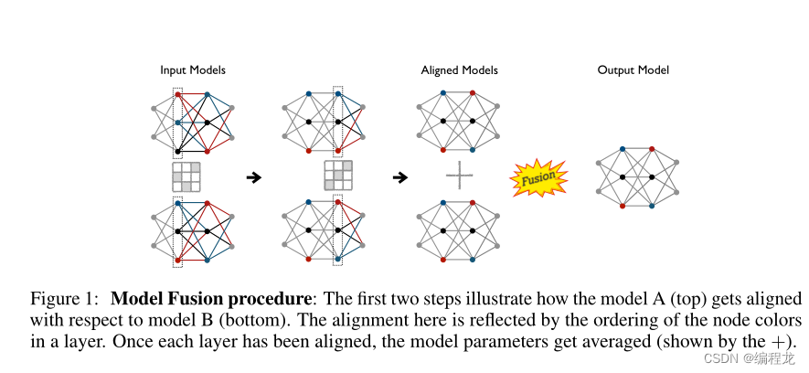
正如在前面的介绍中提到的，参数平均的问题是模型参数之间缺乏一对一的对应关系。特别是对于给定的一层，两种模型的神经元之间没有直接的匹配。例如，这意味着模型A的第$p$个神经元的行为可能与另一个模型B的第$p$个神经元的行为非常不同(就它检测到的特征而言)，相反，在功能上可能与第$p+1$个神经元非常相似。想象一下，如果我们知道神经元之间的完美匹配，那么我们就可以简单地将模型a的神经元相对于模型B的神经元排列起来。这样做之后，对神经元参数进行平均就更有意义了。匹配或赋值可以表述为一个排列矩阵，只需将参数乘以这个矩阵就可以使参数对齐。

但在实践中，对于给定的层，两种模型的神经元之间更有可能存在软对应关系，特别是当它们的数量在两种模型中不相同时。这就是最优传输的作用所在，它以传输图T的形式为我们提供了一个软对齐矩阵。换句话说，对齐问题可以重新表述为，将模型a的给定层中的神经元最优地运输到模型B的同一层中的神经元。

过程： 我们假设模型在$l$层之前的神经元已经排列完成。现在我们定义两个模型在$l$层的概率测度为：${\mu }^{(\ell )}=\left({\mathbf{\alpha }}^{(\ell )},\mathbf{X}[\ell ]\right)$ 以及${\nu }^{(\ell )}=\left({\mathbf{\beta }}^{(\ell )},\mathbf{Y}[\ell ]\right)$。其中$\mathbf{X},\mathbf{Y}$为测量支持。

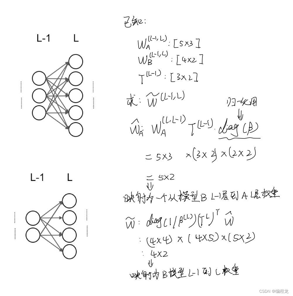
接下来，我们使用均匀分布来初始化每一层的直方图(或概率值)。在实际中，如果使用$n^{(\ell )},m^{(\ell )}$表示为模型A，B在第$\ell$层的大小，那么我们可以得到${\mathbf{\alpha }}^{(\ell )}\leftarrow 1_{n^{(\ell )}}/n^{(\ell )},{\mathbf{\beta }}^{(\ell )}\leftarrow 1_{m^{(\ell )}}/m^{(\ell )}$。现在，根据对齐过程，我们首先对齐当前层的传入边权值。这可以通过与前面的层传输矩阵$T^{(l-1)}$相乘来实现，并且通过相应列边矩阵的倒数${\mathbf{\beta }}^{(\ell -1)}$进行归一化：
$${\hat{\mathbf{W}}}_A^{(\ell ,\ell -1)}\leftarrow {\mathbf{W}}_A^{(\ell ,\ell -1)}{\mathbf{T}}^{(\ell -1)}\mathrm{diag}\left(1/{\mathbf{\beta }}^{(\ell -1)}\right)\text{\hspace{1em}(1)}$$
这里可以这么解释：矩阵${\mathbf{T}}^{(\ell -1)}\mathrm{diag}\left({\mathbf{\beta }}^{-(\ell -1)}\right)$有$m^{(\ell -1)}$个列，因此通过进行和当前权重${\mathbf{W}}_A^{(\ell ,\ell -1)}$的相乘将会产生一个凸组合。

一旦完成了这一步，我们就会专注于校准$\ell$层的神经元。我们假设我们有一个合适的地面度量矩阵$D_{\mathcal{S}}$，我们可以根据${\mu }^{(\ell )},{\nu }^{(\ell )}$以及$\ell$计算最优的传输矩阵${\mathbf{T}}^{(\ell )}$：${\mathbf{T}}^{(\ell )},{\mathcal{W}}_2\leftarrow \mathrm{O}\mathrm{T}\left({\mu }^{(\ell )},{\nu }^{(\ell )},D_{\mathcal{S}}\right)$，其中${\mathcal{W}}_2$表示为Wasserstein距离。现在，我们可以使用这个传输矩阵${\mathbf{T}}^{(\ell )}$来重新排列模型A到模型B的神经元：
$${\tilde{\mathbf{W}}}_A^{(\ell ,\ell -1)}\leftarrow \mathrm{diag}\left(1/{\mathbf{\beta }}^{(\ell )}\right){\mathbf{T}}^{(\ell {)}^{\top }}{\hat{\mathbf{W}}}_A^{(\ell ,\ell -1)}\text{\hspace{1em}(2)}$$
因此，有了这种对齐，我们可以平均两层的权重，以获得融合的权重矩阵$W_{\mathcal{F}}^{(\ell ,\ell -1)}$，如下式：
$${\mathbf{W}}_{\mathcal{F}}^{(\ell ,\ell -1)}\leftarrow \frac{1}{2}\left({\tilde{\mathbf{W}}}_A^{(\ell ,\ell -1)}+{\mathbf{W}}_B^{(\ell ,\ell -1)}\right)\text{\hspace{1em}(3)}$$
注意，由于输入层的顺序对两个模型是相同的，我们从第二层开始对齐。此外，最后一层，也就是输出层，神经元的顺序也是相同的。因此，最后一层的(缩放的)传输映射将等于标识。

多模型融合： 关键思想是，从融合模型的${\mathbf{W}}_{\mathcal{F}}^{(\ell ,\ell -1)}$估计开始，然后根据它对齐所有给定模型，最后返回这些对齐权重的平均值作为融合模型的最终权重。对于两个模型的情况，这相当于我们上面讨论的将融合模型初始化为模型B时的过程，即${\hat{M}}_{\mathcal{F}}\leftarrow M_B$。因为，将模型B与融合模型的这个估计对齐将得到一个等于恒等的(缩放的)传输映射。然后，式(3)将等于返回对齐权重的平均值。

定位策略： 上面我们讨论需要有一个地面度量$D_{\mathcal{S}}$，这里有两种方法可以考虑：

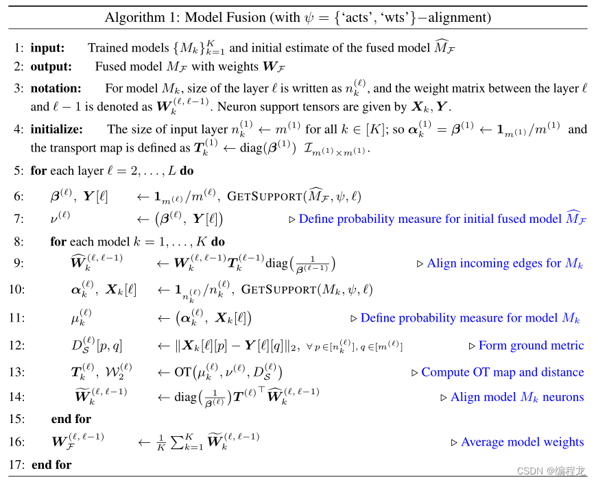
• 基于激活的策略 $(\psi =$ ‘acts’ $)$： 在这个变体中，我们对$m$样本集进行推理， S = { x } i = 1 m S=\{\mathbf{x}\}_{i=1}^m S={x}i=1m​并将所有神经元的激活存储在模型中。因此，我们认为神经元激活，连接到样本的一个向量，作为度量的支持，我们将其表示为${\mathbf{X}}_k\leftarrow \mathrm{ACTS}\left(M_k(S)\right)，\mathbf{Y}\leftarrow \mathrm{ACTS}\left(M_{\mathcal{F}}(S)\right)$。然后，如果两个模型的神经元对给定的样本集产生相似的激活输出，则认为它们是相似的。我们通过计算得到的激活向量之间的欧氏距离来测量这一点。这作为OT计算的基础度量。
• 基于权重的策略($\psi =$ ‘wts’)： 在这里，我们认为每个神经元的支持由传入边的权重给出(堆叠在一个向量中)。因此，一个神经元可以被认为是由权矩阵中与其对应的行表示的。因此，对这种排列类型的度量的支持由，${\mathbf{X}}_k[\ell ]\leftarrow {\hat{\mathbf{W}}}_k^{(\ell ,\ell -1)}，\mathbf{Y}[\ell ]\leftarrow {\hat{\mathbf{W}}}_{\mathcal{F}}^{(\ell ,\ell -1)}$给出。选择这种支持的理由源于特定层的神经元激活被计算为该权重向量与前一层输出之间的内积。OT使用的地面度量是欧氏距离，就像在前面的对齐策略中一样。除了在地面度量中使用实际重量的差异，其余的程序是相同的。

算法如下：

三. 代码解析

论文代码点这里
在开始代码前，我将根据我自己的对文章的理解，然后使用一个简单的例子讲如何根据OT对模型进行融合的：

我们来看代码（为了直观理解，这里选择的是两个MLP模型并且模型大小是一样的，利用MNIST数据集进行考察的），我们首先来看参与进行融合的相关参数

def get_acts_wassersteinized_layers_modularized(args, networks, activations, eps=1e-7, train_loader=None, test_loader=None)
1

其中networks为一个列表，存储了两个模型的对应参数，如下：

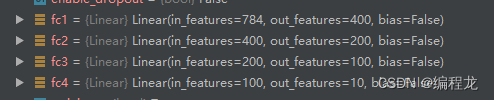
activations存储的是两个模型各层经过数据集得出激活向量组：

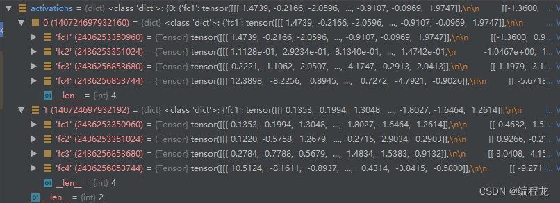
这里选择得batch_size=200，因此每层为：[200,1,400] [200,1,200]等。
接下来我们来看看具体是怎么工作的，首先我们使用均匀分布初始化当前的两个概率向量mu以及nu，如下：

def _get_neuron_importance_histogram(args, layer_weight, is_conv, eps=1e-9):
    print('shape of layer_weight is ', layer_weight.shape)
    if is_conv:
        layer = layer_weight.contiguous().view(layer_weight.shape[0], -1).cpu().numpy()
    else:
        layer = layer_weight.cpu().numpy()
    
    if args.importance == 'l1':
        importance_hist = np.linalg.norm(layer, ord=1, axis=-1).astype(
                    np.float64) + eps
    elif args.importance == 'l2':
        importance_hist = np.linalg.norm(layer, ord=2, axis=-1).astype(
                    np.float64) + eps
    else:
        raise NotImplementedError

    if not args.unbalanced:
        importance_hist = (importance_hist/importance_hist.sum())
        print('sum of importance hist is ', importance_hist.sum())
    # assert importance_hist.sum() == 1.0
    return importance_hist
1
2
3
4
5
6
7
8
9
10
11
12
13
14
15
16
17
18
19
20
21

得到得结果为：

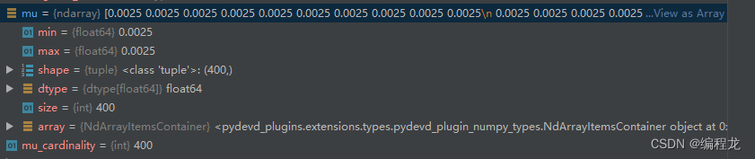
因为当前得层为400，所以1/400=0.025然后填充完成，之后我们计算aligned_w:

if is_conv:
    if args.handle_skips:
        assert len(layer0_shape) == 4
        # save skip_level transport map if there is block ahead
        if layer0_shape[1] != layer0_shape[0]:
            if not (layer0_shape[2] == 1 and layer0_shape[3] == 1):
                print(f'saved skip T_var at layer {idx} with shape {layer0_shape}')
                skip_T_var = T_var.clone()
                skip_T_var_idx = idx
            else:
                print(
                    f'utilizing skip T_var saved from layer layer {skip_T_var_idx} with shape {skip_T_var.shape}')
                # if it's a shortcut (128, 64, 1, 1)
                residual_T_var = T_var.clone()
                residual_T_var_idx = idx  # use this after the skip
                T_var = skip_T_var
            print("shape of previous transport map now is", T_var.shape)
        else:
            if residual_T_var is not None and (residual_T_var_idx == (idx - 1)):
                T_var = (T_var + residual_T_var) / 2
                print("averaging multiple T_var's")
            else:
                print("doing nothing for skips")
    T_var_conv = T_var.unsqueeze(0).repeat(fc_layer0_weight_data.shape[2], 1, 1)
    aligned_wt = torch.bmm(fc_layer0_weight_data.permute(2, 0, 1), T_var_conv).permute(1, 2, 0)

else:
    if fc_layer0_weight.data.shape[1] != T_var.shape[0]:
        # Handles the switch from convolutional layers to fc layers
        # checks if the input has been reshaped
        fc_layer0_unflattened = fc_layer0_weight.data.view(fc_layer0_weight.shape[0], T_var.shape[0],
                                                           -1).permute(2, 0, 1)
        aligned_wt = torch.bmm(
            fc_layer0_unflattened,
            T_var.unsqueeze(0).repeat(fc_layer0_unflattened.shape[0], 1, 1)
        ).permute(1, 2, 0)
        aligned_wt = aligned_wt.contiguous().view(aligned_wt.shape[0], -1)
    else:
        aligned_wt = torch.matmul(fc_layer0_weight.data, T_var)
1
2
3
4
5
6
7
8
9
10
11
12
13
14
15
16
17
18
19
20
21
22
23
24
25
26
27
28
29
30
31
32
33
34
35
36
37
38
39

接下来我们使用激活去计算度量，如下

def process(self, coordinates, other_coordinates=None):
    print('Processing the coordinates to form ground_metric')
    if self.params.geom_ensemble_type == 'wts' and self.params.normalize_wts:
        print("In weight mode: normalizing weights to unit norm")
        coordinates = self._normed_vecs(coordinates)
        if other_coordinates is not None:
            other_coordinates = self._normed_vecs(other_coordinates)

    ground_metric_matrix = self.get_metric(coordinates, other_coordinates)

    if self.params.debug:
        print("coordinates is ", coordinates)
        if other_coordinates is not None:
            print("other_coordinates is ", other_coordinates)
        print("ground_metric_matrix is ", ground_metric_matrix)

    self._sanity_check(ground_metric_matrix)

    ground_metric_matrix = self._normalize(ground_metric_matrix)

    self._sanity_check(ground_metric_matrix)

    if self.params.clip_gm:
        ground_metric_matrix = self._clip(ground_metric_matrix)

    self._sanity_check(ground_metric_matrix)

    if self.params.debug:
        print("ground_metric_matrix at the end is ", ground_metric_matrix)

    return ground_metric_matrix
1
2
3
4
5
6
7
8
9
10
11
12
13
14
15
16
17
18
19
20
21
22
23
24
25
26
27
28
29
30
31

最后利用OT解出T来，并归一化，再使用T排列aligned_w：

T_var = _get_current_layer_transport_map(args, mu, nu, M0, M1, idx=idx, layer_shape=layer_shape, eps=eps, layer_name=layer0_name)
T_var, marginals = _compute_marginals(args, T_var, device, eps=eps)

if args.debug:
    if idx == (num_layers - 1):
        print("there goes the last transport map: \n ", T_var)
        print("and before marginals it is ", T_var/marginals)
    else:
        print("there goes the transport map at layer {}: \n ".format(idx), T_var)

print("Ratio of trace to the matrix sum: ", torch.trace(T_var) / torch.sum(T_var))
print("Here, trace is {} and matrix sum is {} ".format(torch.trace(T_var), torch.sum(T_var)))
setattr(args, 'trace_sum_ratio_{}'.format(layer0_name), (torch.trace(T_var) / torch.sum(T_var)).item())

if args.past_correction:
    print("Shape of aligned wt is ", aligned_wt.shape)
    print("Shape of fc_layer0_weight_data is ", fc_layer0_weight_data.shape)

    t_fc0_model = torch.matmul(T_var.t(), aligned_wt.contiguous().view(aligned_wt.shape[0], -1))
else:
    t_fc0_model = torch.matmul(T_var.t(), fc_layer0_weight_data.view(fc_layer0_weight_data.shape[0], -1))
1
2
3
4
5
6
7
8
9
10
11
12
13
14
15
16
17
18
19
20
21

我们来看看T的形状：

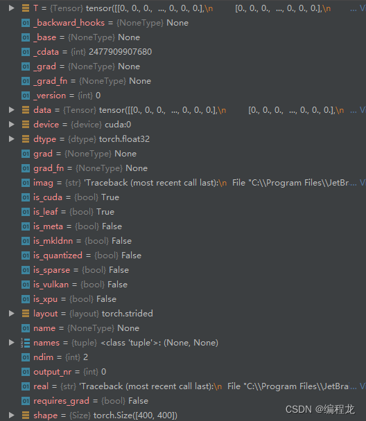
这里是第一层的情况，两个模型的输出都是400*400，所以满足如上。