GCN-LSTM预测道路车辆速度英文 Forecasting using spatio-temporal data with combined Graph Convolution LSTM model_flow direction level traffic flow prediction based

GCN-LSTM模型预测道路交通车辆速度

GCN：又称GNN，图神经网络    LSTM：长短时记忆网络

可做学习参考

Abstract

Accurate traffic prediction is critical for traffic planning, administration, and control in the smart city. However, because of the complicated topological configuration of road and nonlinear traffic patterns, road speed prediction is a difficult job. The research paper aims at looking into taxi speed prediction using GCN-LSTM (a combined model of graph neural network and LSTM). The model can capture the complicated spatial dependence of road nodes on the road network and use LSGC to capture spatial correlation information from the road segment nodes in the road network's K-order local neighbors.

ntroduction

One of the most important tasks in the development of an intelligent transportation management system in a metropolitan area is traffic prediction (Chavhan and Venkataram).  Congestion can raise fuel consumption, pollute the air, and make it difficult to implement public transit plans (Bull). How to accurately estimate future road speeds and give stakeholders with modeling and decision-making tools is likewise a pressing issue for the road management department. In the meanwhile, accurate real - time road speed data is extremely important for individual travelers (Laranjeira). It has the potential to reduce traffic congestion and assist drivers in making informed travel decisions. In terms of estimating speed, volume, density, and travel time, a vast number of techniques have been presented for traffic forecasting. Many statistical approaches, such as support vector machines and the autoregressive integrated moving average (ARIMA) model, have been shown to be useful tools for dealing with time series data (Hayes). These approaches, on the other hand, are unable to capture the spatial-temporal relationship of a road network. Machine learning methods have grown in popularity, and many scholars have been interested in the spatial-temporal characteristics of traffic in recent years (Yoon and Lee).

Traditional machine learning methods, such as support vector regression (SVR) k-nearest neighbor algorithm K-NN (K-Nearest Neighbor), and decision tree models, can delve out the important laws and rich information concealed in traffic flow from massive data and better promote the traffic flow forecasting development process. The advancement of artificial intelligence's potential in traffic prediction has been aided by the creation of deep neural network models. Even though some simple network architectures can enhance model traffic forecast accuracy, they have drawbacks such as sluggish convergence, overfitting, and error values. Recurrent neural networks (RNN), long short-term memory networks (LSTM), and gate recurrent units (GRU) may effectively employ the self-loop system and learn time series characteristics to improve prediction effectiveness when compared to classic neural network models. As a result, it is included in each model to anticipate traffic speed, trip time, and traffic flow, among other things.

Researchers extract spatial features coupled with convolutional neural networks (CNN) from two-dimensional temporal traffic data to capture spatial interdependence in the traffic road network(Zheng et al.). Because the two-dimensional spatiotemporal data used to describe traffic structure is inaccurate and does not conform to the sophisticated road network conditions encountered in real life, some researchers have begun to try to convert the traffic network structure into images and use CNN to understand the traffic images in order to catch the spatial features (mohdsanad). However, the images translated by the traffic network structure contain more or less noise, and the presence of noise will undoubtedly cause CNN to record incorrect spatial correlations.

Because the transportation network may be viewed as a graph with nodes and edges, it has been utilized for dynamic shortest path routing, traffic congestion analysis, and dynamic traffic allocation. The most popular strategy for our graph network research is to establish a spectrum frame in the spectrum domain and build the spectrum convolution based on the plotted graph Laplacian matrix to create the spectrogram convolution model. We use the local spectrogram convolution with polynomial filter to reduce the number of parameters and save calculation time, but the Laplacian matrix power operation still requires a lot of calculation and high complexity, so the Chebyshev polynomial is presented to compute the K-order local convolution, which can reduce the computational computation time from the square level to the linear level. Instead of extracting features from the single-hop neighborhood only, the spectrogram convolution model utilizing Chebyshev polynomial approximation may capture information from the K-order local neighbors of the vertices in the graph, fully taking into consideration the high-order neighborhood of the node.

Graph neural network

Graphs are a type of data structure that can represent a collection of items and their relationships, and are typically represented as nodes and edges (Sharma). Scarselli established the notion of graph neural networks for the first time in and expanded on it in Scarselli GNNs (graph neural networks) are deep learning algorithms that work with graph-structured data(Online et al.). Graphs can be used to represent a wide range of systems in a variety of fields, including social networks, physical systems, knowledge graphs, and a variety of other academic areas. Researchers propose a theoretical framework for measuring the expressive capability of GNNs in capturing various graph topologies and explain how GNNs can be used to handle graph-structured data (Zhou et al.). Because of the astonishing potential of graphs, numerous studies are focusing on understanding graphs using machine learning approaches. The GN defines GN blocks, which are unified neural network components. Each GN block is a "graph-to-graph" module that takes a graph as input, conducts some computations over the structure, and produces a graph as output(Shlomi et al.). The organization of GN blocks in various ways aids the building of complicated designs. Many articles in the subject of traffic flow prediction consider graph-based neural networks to improve forecasting accuracy. Zhang proposes Gated Attention Networks (GaAN) as a unique network architecture for learning on graphs, as well as a unified framework for converting graph aggregators to graph recurrent neural networks(Zhang et al.). Model traffic spatial dependency as a diffusion process on a directed graph, and suggest Diffusion Convolutional Recurrent Neural Network (DCRNN), which can encapsulate both spatial and temporal dependencies between time series.

The graph convolution is generally computed as:

yo∪tVti=1ztiVtjXVtjW,Vtj

Where X(vtj ) is the feature of node vtj . W(·) is a weight function that allocates a weight indexed by the label ℓ(vtj ) from K weights. Zti(vtj ) is the number of the corresponding subset, which normalizes feature representations. Yout(vti) denotes the output of graph convolution at node

Long short term memory

The Long Short Term Memory networks (LSTM) are a type of recurrent neural network (RNN) that can learn long-term dependencies and is used in deep learning (https://www.facebook.com/jason.brownlee.39).  Hochreiter was the first to present it, and it was quickly adopted by a large number of people in subsequent works. Long-term dependency problems are now explicitly addressed by LSTMs, which are particularly well suited to handling time series data. To anticipate network-wide traffic speed, researchers suggested a deep stacked bidirectional and unidirectional LSTM (SBULSTM) neural network architecture that includes both forward and backward dependencies in time series data. Ahybrid model for traffic prediction that combined the Seq2Seq framework with LSTM (“TABLE 1 : Prediction Results for for Linear, CNN, LSTM, CNN-LSTM,...”) is advised. To predict fine-grained traffic conditions, We developed a spatio-temporal long short-term memory network preceded by map-matching. These models estimate the future based on historical data without taking into account the structure of the road network.

Meanwhile, several studies are looking into merging traffic graphs for traffic learning and forecasting (Avila and Mezić). To learn the interactions between roadways in the traffic network and forecast the network-wide traffic status, we offer a unique deep learning framework called Traffic Graph Convolutional Long Short-Term Memory Neural Network (TGC-LSTM). Zhao proposes the temporal graph convolutional network (T-GCN) model, which is used in conjunction with the graph convolutional network (GCN) and gated recurrent unit, as a unique neural network-based traffic forecasting approach (GRU). To answer the multi-link traffic flow forecasting problem, (Wu et al.) offer the Graph Attention LSTM Network (GAT-LSTM) and utilize it to develop an end-to-end trainable encoder-forecaster model. Despite the fact that considerable study has been done on constructing road networks and examining road spatial relations, it is ineffective for capturing road structure properties without a graph.

The GCN-LSTM algorithm.

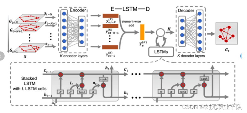
The network structure based on the GCN-LSTM paradigm is primarily encoder-decoder and the steps a GCN-LSTM process is as follows.

Many parallel GCN elements are utilized in the encoder to take out the important features of the graph network with various time series (Zhou et al., “Graph Neural Networks: A Review of Methods and Applications”). The collected time series features are then sent to LSTM, which performs feature analysis and further feature extraction on the sequence data to resolve the data's long-term and short-term dependencies. Finally, the encoder creates and delivers an encoded pair vector to the decoder. The multi-layer feedforward neural network is utilized in the decoder to process the coding vector's features further. Finally, the data is sent to a GCN network, which generates anticipated values.

Experiment

In this traffic flow prediction, we will first, we apply graph convolutional network (GCN) to mine the spatial relationships of traffic flow over multiple observation time steps.

Secondly, we will feed the output of the GCN model to the long short-term memory (LSTM) model which extracts temporal features embedded in traffic flow.

The, we implement a soft attention mechanism on the extracted spatial-temporal traffic features to make final prediction.

We test the proposed method over the Naïve Benchmark method. Experimental results show that the proposed model performs better than the competing methods.

• Data Description

The time steps recorded is 2016. This is from the 207 sensors which records data (speed data) every five minutes. Hence, daily data recorded will be (12daily observations*24hours = 288 observations) in a day.

• Training Process

First, the data is split into two sets, training and testing set. Such that if training takes n number of values from the overall (N) values, the testing will take N-(N-n) number of values. This data’s training size took 80% of the total observations that means 20% was the testing set. This was 1612 as the training set and 404 as the testing set.

After splitting the data into training and testing sets, we can standardize the data in order to make meaningful analysis on it. To transform the data into a more flexible workable range so that our data is meaningful, we transform the data into (0-1) values such that for every feature, the minimum value of that feature gets transformed into a 0, the maximum value gets transformed into a 1, and every other value gets transformed into a decimal between 0 and 1. To achieve this we need to use a library in scikit learn called MinMaxScaler.

Because this is a time series data, we use Minimum and Maximum values in the time series to transform/normalize the test and training set because in time series data using range of values in timesteps will not give you accurate results.

• Data Preprocessing

To feed data into LSTM Model, we first need to prepare the data. This LSTM model works through ‘learning’ from other multiple examples as such, sequences of observations must be passed into the model and this will help LSTM model come up with an output.

Here, 50 minutes of past/historical speed observed was used to help the model predict possible speed in the future. In this work, the first 10 speed records recorded was taken as input and the speed of 1hr worth timesteps (12 timesteps) being the speed we want to predict. Such that we keep shifting by 1 time step and pick the 10 time step window from the current time as input feature the speed one hour ahead of the 10th time step as the output to predict. You keep this up for the entire test data.

• Evaluation Process

The model is fitted 100 number of passes is made in the entire training dataset. This passes are known as epochs. From the query results, we see that a total of 775,239 parameters were passed and out of these, 689,541 was trained and the rest (85,698 parameters) were not.

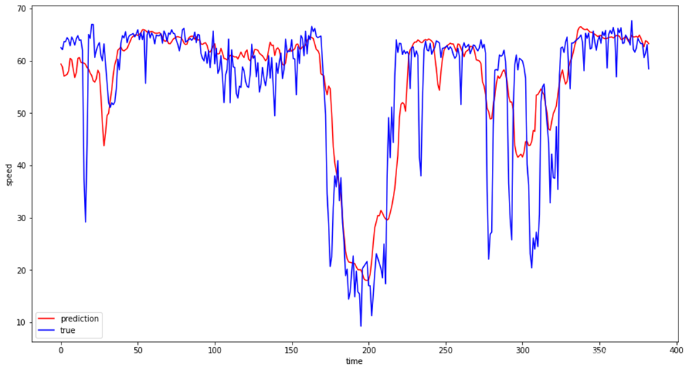
We then check the predicted values using the test dataset. Remember we had split the data into training and testing dataset. It is this test set that is used to check the predictive strength of the model where we can compare the actual verses the predicted values.

The graph below shows the performance of the predicted vs. actual values and as seen they are close. This shows that the model works well.

• Prediction result analysis

The model performance is obtained by using the NN method that is the Neural Network model (GCN-LSTM) by comparing it with the Naïve Benchmark.

 Naïve Benchmark works by predicting whether the same thing that happened previously will happen again and it is good for short term predictions and thus meaningful to use in this case. For the comparison to occur, we fit the Naïve model in the data same way as we did the GCN-LSTM model. We then make a comparison between Artificial Neural Networks (NN) and Naïve Benchmark by using the Mean Absolute Error of each.

The Mean Absolute Error works by giving the difference between the forecasted value and the actual value (Alessandrini). This basically tells us how big of an error we can expect from the forecast on average.

The evaluation index (MSE) calculations formula is as shown below:

MSE=1mI=1nyi-yⅈ2

The trained model is used to predict the test set and calculate the MSE. The smaller the MSE value is, the closer the predicted value of the model is to the real value and the better the generalization ability of the model is.

The results showed that:

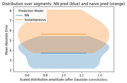
Mean Absolute Error for NN was 3.88

Mean Absolute Error for Naïve was 5.619

This means you can expect more deviation of the forecasted valued from the actual value when you use Naïve prediction as compared to using NN. Generally, this means GCN-LSTM method of prediction is better at spatio-temporal data compared to Naïve prediction.

The graph shows that the NN (GCN-LSTM) model is low compared to the mean absolute error for the Naïve model therefore indicating that GCN-LSTM in fact the preferred method of prediction in this case.

Conclusion

The research focuses on the GCN-LSTM (a combined model of graph neural network and LSTM model for obtaining dynamic attribute features by using the external factor attribute augmentation unit structure. From the K-order local neighbors of the vertices in the graph, this model may describe the geographic properties of traffic flow. The K-order local neighborhood matrix can be used to enlarge the receptive field of the graph convolution, allowing it to extract information from neighbor nodes more precisely. After the data is recovered, the LSTM model is used to capture the time dependence by inputting the characteristic representation of data that changes over time. It solves the inability of previous traffic prediction models by analyzing the effectiveness of the proposed scheme, including the performance analysis of external attribute features and the implementation analysis of various prediction windows, and comparing with different baseline simulations to authenticate the efficiency of the projected approach. External influences impacting traffic flow are taken into account in full.

Works Cited

Alessandrini, Stefano. “Mean Absolute Error - an Overview | ScienceDirect Topics.” Www.sciencedirect.com, 2017, www.sciencedirect.com/topics/engineering/mean-absolute-error.

Avila, A. M., and I. Mezić. “Data-Driven Analysis and Forecasting of Highway Traffic Dynamics.” Nature Communications, vol. 11, no. 1, 29 Apr. 2020, 10.1038/s41467-020-15582-5. Accessed 9 June 2021.

Bull, Alberto. Publicaciones de La CEPAL. 2003.

Chavhan, Suresh, and Pallapa Venkataram. “Prediction Based Traffic Management in a Metropolitan Area.” Journal of Traffic and Transportation Engineering (English Edition), July 2019, www.sciencedirect.com/science/article/pii/S209575641730524X, 10.1016/j.jtte.2018.05.003.

Hayes, Adam. “Autoregressive Integrated Moving Average (ARIMA).” Investopedia, 2019, www.investopedia.com/terms/a/autoregressive-integrated-moving-average-arima.asp.

https://www.facebook.com/jason.brownlee.39. “A Gentle Introduction to Long Short-Term Memory Networks by the Experts.” Machine Learning Mastery, 19 July 2017, machinelearningmastery.com/gentle-introduction-long-short-term-memory-networks-experts/.

Laranjeira, Joao. “What Is Traffic Prediction and How Does It Work? | TomTom Blog.” TomTom, www.tomtom.com/blog/traffic-and-travel-information/road-traffic-prediction/.

Melodia, Tommaso, and Antonio Iera. “Computer Networks | ScienceDirect.com.” Sciencedirect.com, 2019, www.sciencedirect.com/journal/computer-networks. Accessed 18 Apr. 2019.

mohdsanad. “CNN Image Classification | Image Classification Using CNN.” Analytics Vidhya, 18 Feb. 2020, www.analyticsvidhya.com/blog/2020/02/learn-image-classification-cnn-convolutional-neural-networks-3-datasets/.

Online, Research, et al. The Graph Neural Network Model the Graph Neural Network Model. 2009.

Sharma, Rohit. “Graphs in Data Structure: Types, Storing & Traversal.” UpGrad Blog, 7 Oct. 2020, www.upgrad.com/blog/graphs-in-data-structure/.

Shlomi, Jonathan, et al. “Graph Neural Networks in Particle Physics.” Machine Learning: Science and Technology, vol. 2, no. 2, 8 Jan. 2021, p. 021001, 10.1088/2632-2153/abbf9a. Accessed 14 July 2021.

“TABLE 1 : Prediction Results for for Linear, CNN, LSTM, CNN-LSTM,...” ResearchGate, www.researchgate.net/figure/Prediction-results-for-for-Linear-CNN-LSTM-CNN-LSTM-Improved-CNN-LSTM-models_tbl1_325706226. Accessed 19 Apr. 2022.

“Traffic Flow Prediction - an Overview | ScienceDirect Topics.” Www.sciencedirect.com, www.sciencedirect.com/topics/computer-science/traffic-flow-prediction. Accessed 19 Apr. 2022.

Wu, Tianlong, et al. “Graph Attention LSTM Network: A New Model for Traffic Flow Forecasting.” IEEE Xplore, 1 July 2018, ieeexplore.ieee.org/document/8612556. Accessed 19 Apr. 2022.

Yoon, Junho, and Sugie Lee. “Spatio-Temporal Patterns in Pedestrian Crashes and Their Determining Factors: Application of a Space-Time Cube Analysis Model.” Accident Analysis & Prevention, vol. 161, 1 Oct. 2021, p. 106291, www.sciencedirect.com/science/article/abs/pii/S0001457521003225?via%3Dihub, 10.1016/j.aap.2021.106291.

Zhang, Jiani, et al. “GaAN: Gated Attention Networks for Learning on Large and Spatiotemporal Graphs.” ArXiv:1803.07294 [Cs], 20 Mar. 2018, arxiv.org/abs/1803.07294. Accessed 19 Apr. 2022.

Zheng, Yan, et al. “Traffic Volume Prediction: A Fusion Deep Learning Model Considering Spatial–Temporal Correlation.” Sustainability, vol. 13, no. 19, 24 Sept. 2021, p. 10595, 10.3390/su131910595. Accessed 5 Dec. 2021.

Zhou, Jie, et al. “Graph Neural Networks: A Review of Methods and Applications.” AI Open, vol. 1, 2020, pp. 57–81, arxiv.org/ftp/arxiv/papers/1812/1812.08434.pdf, 10.1016/j.aiopen.2021.01.001.

---. “Graph Neural Networks: A Review of Methods and Applications.” AI Open, vol. 1, 2020, pp. 57–81, arxiv.org/ftp/arxiv/papers/1812/1812.08434.pdf, 10.1016/j.aiopen.2021.01.001.