Regression算法

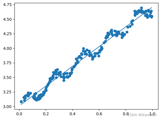
用线性回归找到最佳拟合直线

from google.colab import drive
drive.mount("/content/drive")
1
2

Mounted at /content/drive
1

from numpy import *
1

def loadDataSet(fileName):
  numFeat = len(open(fileName).readline().split('\t')) - 1
  dataMat = []
  labelMat = []
  fr = open(fileName)
  for line in fr.readlines():
    lineArr = []
    curLine = line.strip().split('\t')
    for i in range(numFeat):
      lineArr.append(float(curLine[i]))
    dataMat.append(lineArr)
    labelMat.append(float(curLine[-1]))
  return dataMat, labelMat
1
2
3
4
5
6
7
8
9
10
11
12
13

这段代码定义了一个名为loadDataSet的函数，用于加载数据集并将其分为特征矩阵和标签向量。以下是对该函数的代码分析：

def loadDataSet(fileName):
    numFeat = len(open(fileName).readline().split('\t')) - 1
    dataMat = []
    labelMat = []
    fr = open(fileName)
    for line in fr.readlines():
        lineArr = []
        curLine = line.strip().split('\t')
        for i in range(numFeat):
            lineArr.append(float(curLine[i]))
        dataMat.append(lineArr)
        labelMat.append(float(curLine[-1]))
    return dataMat, labelMat
1
2
3
4
5
6
7
8
9
10
11
12
13

1. numFeat = len(open(fileName).readline().split('\t')) - 1

   • 通过打开文件并读取第一行，计算特征的数量。这里假设数据集是用 tab 分隔的文本文件，每一行的最后一个元素是标签。

2. dataMat = [] 和 labelMat = []

   • 创建空列表，用于存储特征矩阵和标签向量。

3. fr = open(fileName)

   • 打开文件以供读取。

4. for line in fr.readlines():

   • 遍历文件的每一行。

5. lineArr = []

   • 创建一个空列表，用于存储每行的特征数据。

6. curLine = line.strip().split('\t')

   • 去除行首尾的空白符，然后按制表符分割字符串，得到当前行的特征和标签。

7. for i in range(numFeat):

   • 遍历特征的数量。

8. lineArr.append(float(curLine[i]))

   • 将当前行的特征值转换为浮点数并添加到 lineArr 中。

9. dataMat.append(lineArr) 和 labelMat.append(float(curLine[-1]))

   • 将特征数据添加到 dataMat 列表中，将标签值添加到 labelMat 列表中。

10. return dataMat, labelMat

    • 返回特征矩阵和标签向量作为元组。

该函数的作用是从文件中读取数据集，并将其分为特征矩阵和标签向量。

标准回归函数

def standRegres(xArr, yArr):
  xMat = mat(xArr)
  yMat = mat(yArr).T
  xTx = xMat.T * xMat
  if linalg.det(xTx) == 0:
    print("This matrix is singular, cannot do inverse")
    return
  ws = xTx.I * (xMat.T * yMat)
  return ws
1
2
3
4
5
6
7
8
9

这段代码是用于实现普通最小二乘线性回归（OLS）的 Python 函数。下面是对函数的代码分析：

1. def standRegres(xArr, yArr):

   • 函数的定义，它接受两个参数：xArr是一个列表或数组，包含输入特征的数据集；yArr是一个列表或数组，包含对应的目标变量值。

2. xMat = mat(xArr)

   • 将输入特征数据集转换为一个 NumPy 矩阵。

3. yMat = mat(yArr).T

   • 将目标变量数据集转换为一个 NumPy 矩阵，并且将其转置，以确保其为列向量。

4. xTx = xMat.T * xMat

   • 计算特征数据矩阵的转置与其自身的乘积。这是用来计算线性回归系数的一个步骤。

5. if linalg.det(xTx) == 0:

   • 使用线性代数库（linalg）中的det()函数计算矩阵xTx的行列式（Determinant）。如果行列式为0，则说明矩阵不可逆（singular），这种情况下无法求解线性回归，因此打印错误消息并返回。

6. ws = xTx.I * (xMat.T * yMat)

   • 如果矩阵可逆，那么使用矩阵的逆（I）乘以特征矩阵转置与目标变量矩阵的乘积来计算回归系数（weights）。

7. return ws

   • 返回计算得到的回归系数。

该函数实现了基本的线性回归，通过计算输入特征与目标变量之间的关系，得出一个线性模型，用于预测目标变量的值。

xArr, yArr = loadDataSet('/content/drive/MyDrive/Colab Notebooks/MachineLearning/《机器学习实战》/06丨预测数值型数据：回归/用线性回归找到最佳拟合直线/ex0.txt')
1

xArr[:2]
1

[[1.0, 0.067732], [1.0, 0.42781]]
1

ws = standRegres(xArr, yArr)
1

ws
1

matrix([[3.00774324],
        [1.69532264]])
1
2

xMat = mat(xArr)
yMat = mat(yArr)
yHat = xMat * ws
1
2
3

import matplotlib.pyplot as plt
fig = plt.figure()
ax = fig.add_subplot(111)
ax.scatter(xMat[:,1].flatten().A[0], yMat.T[:,0].flatten().A[0])
xCopy = xMat.copy()
xCopy.sort(0)
yHat = xCopy*ws
ax.plot(xCopy[:,1], yHat)
plt.show()
1
2
3
4
5
6
7
8
9

yHat = xMat*ws
1

yHat.shape
1

(200, 1)
1

yMat.shape
1

(1, 200)
1

corrcoef(yHat.T, yMat)
1

array([[1.        , 0.98647356],
       [0.98647356, 1.        ]])
1
2

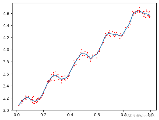
局部加权线性回归函数

def lwlr(testPoint, xArr, yArr, k=1.0):
  xMat = mat(xArr)
  yMat = mat(yArr).T
  m = shape(xMat)[0]
  weights = mat(eye(m))
  for j in range(m):
    diffMat = testPoint - xMat[j, :]
    weights[j, j] = exp(diffMat*diffMat.T/(-2.0*k**2))
  xTx = xMat.T * (weights * xMat)
  if linalg.det(xTx) == 0.0:
    print("This matrix is singular, cannot do inverse")
    return
  ws = xTx.I * (xMat.T * (weights * yMat))
  return testPoint * ws
1
2
3
4
5
6
7
8
9
10
11
12
13
14

这段代码实现了局部加权线性回归（Locally Weighted Linear Regression，LWLR）的函数。以下是对该函数的代码分析：

1. def lwlr(testPoint, xArr, yArr, k=1.0):

   • 函数的定义，它接受四个参数：testPoint是待预测的数据点；xArr是一个列表或数组，包含输入特征的数据集；yArr是一个列表或数组，包含对应的目标变量值；k是一个可选参数，控制权重的带宽，默认为1.0。

2. xMat = mat(xArr)

   • 将输入特征数据集转换为一个 NumPy 矩阵。

3. yMat = mat(yArr).T

   • 将目标变量数据集转换为一个 NumPy 矩阵，并且将其转置，以确保其为列向量。

4. m = shape(xMat)[0]

   • 获取输入特征矩阵的行数，即数据集中样本的数量。

5. weights = mat(eye(m))

   • 创建一个单位矩阵作为权重矩阵，其大小为$m\times m$，其中$m$为数据集中样本的数量。

6. for j in range(m):

   • 遍历数据集中的每个样本。

7. diffMat = testPoint - xMat[j, :]

   • 计算测试点与当前样本之间的差值。

8. weights[j, j] = exp(diffMat*diffMat.T/(-2.0*k**2))

   • 计算当前样本的权重，利用高斯核函数，其中 $exp$ 是指数函数，$k$ 是带宽参数。

9. xTx = xMat.T * (weights * xMat)

   • 计算加权的特征矩阵的转置与自身的乘积。

10. if linalg.det(xTx) == 0.0:

    • 检查加权特征矩阵的行列式是否为0，如果是则无法求逆，打印错误消息并返回。

11. ws = xTx.I * (xMat.T * (weights * yMat))

    • 如果加权特征矩阵可逆，那么使用矩阵的逆（I）乘以加权特征矩阵转置与目标变量矩阵的乘积来计算回归系数。

12. return testPoint * ws

    • 返回测试点与计算得到的回归系数的乘积，即用局部加权线性回归模型对测试点进行预测。

该函数实现了局部加权线性回归，它对于每个测试点都会根据其附近的数据点赋予不同的权重，以更好地拟合局部数据。

def lwlrTest(testArr, xArr, yArr, k=1.0):
  m = shape(testArr)[0]
  yHat = zeros(m)
  for i in range(m):
    yHat[i] = lwlr(testArr[i], xArr, yArr, k)
  return yHat
1
2
3
4
5
6

xArr, yArr = loadDataSet('/content/drive/MyDrive/Colab Notebooks/MachineLearning/《机器学习实战》/06丨预测数值型数据：回归/用线性回归找到最佳拟合直线/ex0.txt')
1

yArr[0]
1

3.176513
1

lwlr(xArr[0], xArr, yArr, 1.0)
1

<ipython-input-27-f0eaaa458f3a>:8: DeprecationWarning: Conversion of an array with ndim > 0 to a scalar is deprecated, and will error in future. Ensure you extract a single element from your array before performing this operation. (Deprecated NumPy 1.25.)
  weights[j, j] = exp(diffMat*diffMat.T/(-2.0*k**2))

matrix([[3.12204471]])
1
2
3
4

lwlr(xArr[0], xArr, yArr, 0.001)
1

<ipython-input-27-f0eaaa458f3a>:8: DeprecationWarning: Conversion of an array with ndim > 0 to a scalar is deprecated, and will error in future. Ensure you extract a single element from your array before performing this operation. (Deprecated NumPy 1.25.)
  weights[j, j] = exp(diffMat*diffMat.T/(-2.0*k**2))

matrix([[3.20175729]])
1
2
3
4

yHat = lwlrTest(xArr, xArr, yArr, 0.01)
1

<ipython-input-27-f0eaaa458f3a>:8: DeprecationWarning: Conversion of an array with ndim > 0 to a scalar is deprecated, and will error in future. Ensure you extract a single element from your array before performing this operation. (Deprecated NumPy 1.25.)
  weights[j, j] = exp(diffMat*diffMat.T/(-2.0*k**2))
<ipython-input-28-3481d8d2a021>:5: DeprecationWarning: Conversion of an array with ndim > 0 to a scalar is deprecated, and will error in future. Ensure you extract a single element from your array before performing this operation. (Deprecated NumPy 1.25.)
  yHat[i] = lwlr(testArr[i], xArr, yArr, k)
1
2
3
4

xMat = mat(xArr)
srtInd = xMat[:,1].argsort(0)
xSort = xMat[srtInd][:,0,:]
1
2
3

import matplotlib.pyplot as plt
fig = plt.figure()
ax = fig.add_subplot(111)
ax.plot(xSort[:,1], yHat[srtInd])
ax.scatter(xMat[:,1].flatten().A[0], mat(yArr).T.flatten().A[0], s=2, c='red')
plt.show()
1
2
3
4
5
6