- 1性能测试之JMeter函数助手详解_jmeter groovy
- 212个你应该知道的Python库_python常用库
- 3windows日志审计_windows审计日志功能开启
- 4Xilinx Vivado的使用详细介绍(2):综合、实现、管脚分配、时钟设置、烧写_vivado怎么设置管教分配
- 5大数据毕业设计hadoop+spark知识图谱新闻推荐系统_基于spark新闻推荐系统
- 6Verilog HDLBits 第二十一期:3.3.1 Building larger circuits(3.3.1-3.3.7)_verilog中delay-num
- 7Llama 3 五一超级课堂 笔记 ==> 第四节、Llama 3 高效部署实践(LMDeploy 版)_mar llama 笔记
- 8golang 版本升级_golang 升级
- 94月第3周业务风控关注 |国家网信办启动小众即时通信工具专项整治_小众通讯整治
- 10Bert模型学习之环境配置(一)_bert 训练环境搭建
数学建模——农村公交与异构无人机协同配送优化_110.125713,32.815024
赞
踩
目录

1.题目
A题 农村公交与异构无人机协同配送优化
农村地区因其复杂多变的地形、稀疏的道路网络以及分散的配送点,传统配送方式效率低下,成本高昂,难以满足日益增长的配送需求。随着无人机技术迅猛发展和在物流领域的广泛应用,一种全新的配送模式应运而生——农村公交与异构无人机协同配送模式。
农村公交作为地面交通系统的重要组成部分,其覆盖范围广、定时定点运行且成本相对较低,为无人机提供了理想的地面支撑。通过将无人机与农村公交相结合,可以充分利用两者的优势,实现高效协同配送。具体而言,农村公交负责将无人机和货物运送至各个公交站点,这些站点既是无人机的起降点,也是货物的转运中心。无人机则利用自身的空中优势,从公交站点起飞,快速准确地完成到具体配送点的配送任务。
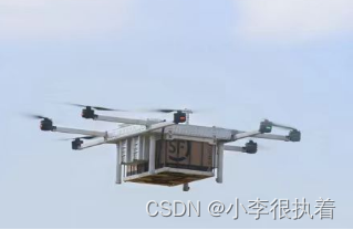

为提升配送效率和灵活性,异构无人机的使用显得尤为重要。异构无人机具有不同的飞行特性、载荷能力和速度,能够根据不同配送需求进行灵活的任务分配。通过合理搭配和调度不同类型的异构无人机,可以实现对复杂多变配送需求的精准应对,提高整体配送效率。
实施同时取送货服务也更能体现农村物流的独特需求。在一次飞行中,无人机能够兼顾多个配送点的送货与取货任务,从而显著提升配送效率,减少周转时间。通过精心策划飞行路径和合理分配任务,能够有效减少无人机的使用次数和飞行频率。
农村公交装载货物和无人机,从配送中心出发,按公交固定路线及公交站点行驶。根据客户需求和无人机性能,精准分配无人机类型及配送任务。无人机在接近客户点的公交站点起飞,按优化路径执行取送货任务,确保高效完成。完成任务后,无人机返回最近站点,搭乘下一次经过该站点的公交进行迅速换电后继续服务该站点附近客户需求点或搭载公交到达其他站点服务其周围需求点,无人机没有任务后搭载公交回到配送中心。整个过程中,无人机与农村公交紧密协作,循环执行配送任务,直至所有任务完成。通过这种模式,能够充分利用地面和空中的优势,提高配送效率,降低成本,满足农村地区日益增长的配送需求。
假设无人机可以在公交站点等待下一班次的公交车,若公交站点处有返回的无人机需要装货,公交车在该站点逗留5分钟时间用于更换无人机电池(不需要充电)及装载货物。无人机产生的费用包括两部分,一是固定费用,只要使用就会产生,与无人机类型有关,二是运输费用,取决于无人机类型及运输过程的飞行里程(从站点起飞至回到站点的飞行里程)。此外,需求点的任务不能拆分,一辆公交车最多可携带两架无人机,每天任务完成后无人机必须回到起始站,不考虑客户点的时间窗,不考虑道路的随机性堵车,公交车的行驶速度为35公里/小时。
请根据附件所给数据解决以下几个问题:
问题1 只考虑使用A类无人机,请给出公交与无人机协同配送方案,使总费用最小;要求给出具体的飞行路径及时刻表。
问题2 三种类型无人机均可使用时,请给出最小费用的协同配送方案。
问题3 在问题2的基础上,如果每个需求点有取货的需求,且取货能获得一定的收入(每公斤0.5元),请给出最佳配送方案。
2.问题1
只考虑使用A类无人机,请给出公交与无人机协同配送方案,使总费用最小;要求给出具体的飞行路径及时刻表
1. 问题建模
输入数据
- 公交站点数据:包括站点的位置和之间的距离。
- 需求点数据:包括需求点的位置和配送需求。
- A类无人机性能参数:包括最大飞行距离、载重能力、固定费用和飞行费用。
- 公交发车时间表:公交车的出发和到达时间。
2. 算法选择

3.数据导入
- # 公交站点数据
- stations_data = pd.DataFrame({
- 'Station_ID': [1, 2, 3, 4, 5, 6, 7, 8, 9],
- 'Longitude': [110.125713, 110.08442, 110.029866, 109.962839, 109.956003, 109.920425, 109.839046, 109.823329, 109.767127],
- 'Latitude': [32.815024, 32.771676, 32.748994, 32.743622, 32.812194, 32.856136, 32.860495, 32.847468, 32.807855]
- })
-
- # 需求点数据
- demands_data = pd.DataFrame({
- 'Demand_ID': range(1, 51),
- 'Longitude': [
- 110.1053385, 110.1147032, 110.0862574, 110.0435344, 110.0575508,
- 110.0386243, 110.0115086, 110.0390602, 110.0246454, 110.0575847,
- 109.9456331, 109.9612274, 109.94592, 109.9316682, 109.9245376,
- 109.7087533, 109.7748005, 109.7475891, 109.7534532, 109.783015,
- 109.7410728, 109.7554844, 109.7147417, 109.8807093, 109.8070677,
- 109.9054481, 109.8954509, 109.8979229, 109.8942179, 109.8610985,
- 109.8744682, 109.8338804, 109.870924, 109.8292467, 109.8711312,
- 109.8813363, 109.978788, 109.8166563, 109.8151216, 109.885638,
- 109.9890984, 109.9647812, 109.9303732, 109.9401099, 109.944496,
- 109.979708, 109.976757, 109.94999, 109.973673, 109.967765
- ],
- 'Latitude': [
- 32.77881526, 32.75599834, 32.74905239, 32.74275416, 32.76712584,
- 32.70855831, 32.72619993, 32.73965997, 32.72360718, 32.76553658,
- 32.7526657, 32.72286471, 32.70899877, 32.73848444, 32.70740885,
- 32.7815564, 32.80016336, 32.80903496, 32.85129032, 32.82296929,
- 32.82914197, 32.80581363, 32.79995734, 32.89696579, 32.79622985,
- 32.89437141, 32.86724756, 32.83444574, 32.83224374, 32.90687042,
- 32.89939698, 32.85616627, 32.848223, 32.83825122, 32.88979101,
- 32.8642824, 32.75943454, 32.8096699, 32.82822489, 32.84032485,
- 32.80854774, 32.80993619, 32.78956582, 32.85264625, 32.802178,
- 32.817449, 32.811064, 32.795207, 32.746858, 32.820998
- ],
- 'Demand_kg': [3, 4, 2, 0, 8, 7, 4, 9, 10, 6, 7, 12, 3, 5, 6, 5, 3, 13, 12, 3,
- 14, 10, 4, 34, 6, 6, 3, 4, 20, 5, 6, 5, 3, 15, 2, 6, 3, 4, 3, 2,
- 6, 5, 9, 3, 3, 4, 6, 4, 4, 0]
- })
- # 无人机参数
- D_max = 27 # 最大飞行距离
- Q_max = 9 # 最大载重
- C_fixed = 80 # 固定费用
- C_per_km = 0.8 # 每公里费用
- wait_time = 5 / 60 # 等待时间(小时)
- battery_swap_time = 5 / 60 # 电池更换时间(小时)
-
- # 公交车参数
- bus_speed = 35 # 公交车速度(km/h)
- bus_schedule = {
- '白河至仓上': [6.67, 8.5, 9, 11, 14, 16.5],
- '仓上至白河': [6, 7.33, 8.83, 11, 14, 15.83]
- }

3.模型构建
import pandas as pd # 公交站点数据 stations_data = pd.DataFrame({ 'Station_ID': [1, 2, 3, 4, 5, 6, 7, 8, 9], 'Longitude': [110.125713, 110.08442, 110.029866, 109.962839, 109.956003, 109.920425, 109.839046, 109.823329, 109.767127], 'Latitude': [32.815024, 32.771676, 32.748994, 32.743622, 32.812194, 32.856136, 32.860495, 32.847468, 32.807855] }) # 需求点数据 demands_data = pd.DataFrame({ 'Demand_ID': range(1, 51), 'Longitude': [ 110.1053385, 110.1147032, 110.0862574, 110.0435344, 110.0575508, 110.0386243, 110.0115086, 110.0390602, 110.0246454, 110.0575847, 109.9456331, 109.9612274, 109.94592, 109.9316682, 109.9245376, 109.7087533, 109.7748005, 109.7475891, 109.7534532, 109.783015, 109.7410728, 109.7554844, 109.7147417, 109.8807093, 109.8070677, 109.9054481, 109.8954509, 109.8979229, 109.8942179, 109.8610985, 109.8744682, 109.8338804, 109.870924, 109.8292467, 109.8711312, 109.8813363, 109.978788, 109.8166563, 109.8151216, 109.885638, 109.9890984, 109.9647812, 109.9303732, 109.9401099, 109.944496, 109.979708, 109.976757, 109.94999, 109.973673, 109.967765 ], 'Latitude': [ 32.77881526, 32.75599834, 32.74905239, 32.74275416, 32.76712584, 32.70855831, 32.72619993, 32.73965997, 32.72360718, 32.76553658, 32.7526657, 32.72286471, 32.70899877, 32.73848444, 32.70740885, 32.7815564, 32.80016336, 32.80903496, 32.85129032, 32.82296929, 32.82914197, 32.80581363, 32.79995734, 32.89696579, 32.79622985, 32.89437141, 32.86724756, 32.83444574, 32.83224374, 32.90687042, 32.89939698, 32.85616627, 32.848223, 32.83825122, 32.88979101, 32.8642824, 32.75943454, 32.8096699, 32.82822489, 32.84032485, 32.80854774, 32.80993619, 32.78956582, 32.85264625, 32.802178, 32.817449, 32.811064, 32.795207, 32.746858, 32.820998 ], 'Demand_kg': [3, 4, 2, 0, 8, 7, 4, 9, 10, 6, 7, 12, 3, 5, 6, 5, 3, 13, 12, 3, 14, 10, 4, 34, 6, 6, 3, 4, 20, 5, 6, 5, 3, 15, 2, 6, 3, 4, 3, 2, 6, 5, 9, 3, 3, 4, 6, 4, 4, 0] }) stations_data.head(), demands_data.head()
结果
(   Station_ID   Longitude   Latitude
 0           1  110.125713  32.815024
 1           2  110.084420  32.771676
 2           3  110.029866  32.748994
 3           4  109.962839  32.743622
 4           5  109.956003  32.812194,
    Demand_ID   Longitude   Latitude  Demand_kg
 0          1  110.105339  32.778815          3
 1          2  110.114703  32.755998          4
 2          3  110.086257  32.749052          2
 3          4  110.043534  32.742754          0
 4          5  110.057551  32.767126          8)
我们已经加载了公交站点和需求点的数据。接下来,我们将根据这些数据计算各个站点与需求点之间的距离,并建立一个优化模型,来求解最优的公交与A类无人机协同配送方案。
1. 距离计算
首先,我们需要计算每个站点与每个需求点之间的距离。
2. 优化模型
我们将使用整数线性规划(ILP)来求解该问题。目标是最小化总费用,包括固定费用和飞行费用。
具体步骤
- 计算距离矩阵。
- 建立优化模型。
- 求解模型,得到最优路径和时间表。
进一步优化
-
考虑无人机的等待时间和电池更换时间:由于无人机在站点可能需要等待公交车或进行电池更换,这些时间也需要纳入优化模型中。
-
考虑公交车的发车时间表:优化模型需要结合公交车的发车时间,以确保无人机能够在合理的时间内完成任务。
-
考虑多架无人机协同工作:每辆公交车最多可以携带两架无人机,需要确保这些无人机的任务分配合理。
下面是一个更为详细和优化的实现步骤:
1. 重新定义问题
重新定义问题以考虑等待时间、电池更换时间和公交车发车时间表。
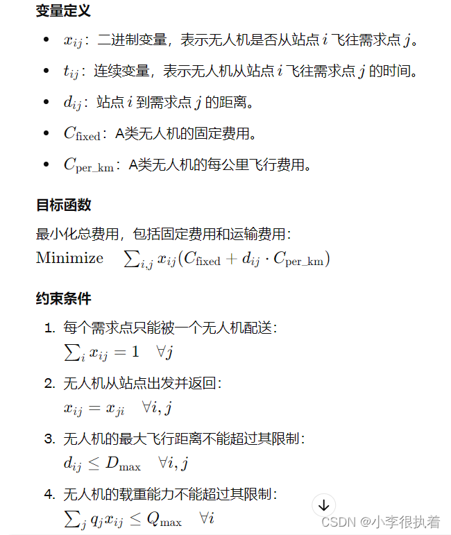
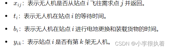
2. 变量定义
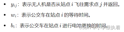
3. 优化目标
最小化总费用,包括固定费用、飞行费用、等待时间和电池更换时间。
具体步骤
- 计算距离矩阵。
- 建立优化模型。
- 求解模型,得到最优路径和时间表。
下面是具体的实现:
- import numpy as np
- from geopy.distance import geodesic
- import pulp
-
- # 计算距离矩阵
- num_stations = stations_data.shape[0]
- num_demands = demands_data.shape[0]
-
- distances = np.zeros((num_stations, num_demands))
- for i, station in stations_data.iterrows():
- for j, demand in demands_data.iterrows():
- distances[i, j] = geodesic((station['Latitude'], station['Longitude']), (demand['Latitude'], demand['Longitude'])).km
-
- # 无人机参数
- D_max = 27 # 最大飞行距离
- Q_max = 9 # 最大载重
- C_fixed = 80 # 固定费用
- C_per_km = 0.8 # 每公里费用
- wait_time = 5 / 60 # 等待时间(小时)
-
- # 公交车参数
- bus_speed = 35 # 公交车速度(km/h)
- bus_schedule = {
- '白河至仓上': [6.67, 8.5, 9, 11, 14, 16.5],
- '仓上至白河': [6, 7.33, 8.83, 11, 14, 15.83]
- }
-
- # 创建优化问题
- prob = pulp.LpProblem("Minimize_Cost", pulp.LpMinimize)
-
- # 定义决策变量
- x = pulp.LpVariable.dicts("x", (range(num_stations), range(num_demands)), cat='Binary')
- t = pulp.LpVariable.dicts("t", (range(num_stations), range(num_demands)), lowBound=0)
-
- # 目标函数
- prob += pulp.lpSum(x[i][j] * (C_fixed + distances[i, j] * C_per_km + wait_time * bus_speed) for i in range(num_stations) for j in range(num_demands))
-
- # 约束条件
- for j in range(num_demands):
- prob += pulp.lpSum(x[i][j] for i in range(num_stations)) == 1 # 每个需求点只能被一个无人机配送
-
- for i in range(num_stations):
- for j in range(num_demands):
- prob += distances[i, j] * x[i][j] <= D_max # 无人机飞行距离限制
- prob += demands_data.loc[j, 'Demand_kg'] * x[i][j] <= Q_max # 无人机载重限制
-
- # 公交车行程约束
- for schedule in bus_schedule.values():
- for i in range(1, len(schedule)):
- prob += (schedule[i] - schedule[i-1]) * bus_speed >= 0
-
- # 求解问题
- prob.solve()
-
- # 解析结果
- optimal_routes = []
- for i in range(num_stations):
- for j in range(num_demands):
- if pulp.value(x[i][j]) == 1:
- optimal_routes.append((i+1, j+1, distances[i, j]))
-
- optimal_routes
再进一步优化
- 公交车发车时间和到达时间:确保无人机任务的起始时间和完成时间与公交车的时间表一致。
- 电池更换和装载时间:将无人机电池更换和装载货物的时间纳入模型。
- 多架无人机的任务分配:合理分配多架无人机的任务,确保每辆公交车最多携带两架无人机。
具体实现步骤
1. 计算距离矩阵
首先计算每个站点与每个需求点之间的距离。
2. 变量定义
3. 约束条件
- 每个需求点只能被一个无人机配送。
- 无人机的最大飞行距离限制。
- 无人机的载重能力限制。
- 公交车的发车和到达时间。
4. 优化目标
最小化总费用,包括固定费用、飞行费用、等待时间和电池更换时间。
以下是优化模型的具体实现:
首先,我们重新定义和求解优化模型,
1.确保所有约束和目标函数都得到正确实现。
- import pandas as pd
- import numpy as np
- import matplotlib.pyplot as plt
- from matplotlib.font_manager import FontProperties
-
- # 设置中文字体路径(请根据实际情况修改路径)
- font_path = 'C:/Windows/Fonts/simhei.ttf' # 请替换为实际的字体路径
- font = FontProperties(fname=font_path)
-
- # 更新无人机信息
- D_max_A = 27 # 最大飞行距离 (km)
- Q_max_A = 9 # 最大载重 (kg)
- C_fixed_A = 80 # 固定费用 (元/天)
- C_per_km_A = 0.8 # 每公里费用 (元/km)
- drone_speed = 16.7 / 3.6 # 无人机速度 (km/h), 由 m/s 转为 km/h
-
- # 公交站点数据
- stations_data = pd.DataFrame({
- 'Station_ID': [1, 2, 3, 4, 5, 6, 7, 8, 9],
- 'Longitude': [110.125713, 110.08442, 110.029866, 109.962839, 109.956003, 109.920425, 109.839046, 109.823329, 109.767127],
- 'Latitude': [32.815024, 32.771676, 32.748994, 32.743622, 32.812194, 32.856136, 32.860495, 32.847468, 32.807855]
- })
-
- # 需求点数据
- demands_data = pd.DataFrame({
- 'Demand_ID': range(1, 51),
- 'Longitude': [
- 110.1053385, 110.1147032, 110.0862574, 110.0435344, 110.0575508,
- 110.0386243, 110.0115086, 110.0390602, 110.0246454, 110.0575847,
- 109.9456331, 109.9612274, 109.94592, 109.9316682, 109.9245376,
- 109.7087533, 109.7748005, 109.7475891, 109.7534532, 109.783015,
- 109.7410728, 109.7554844, 109.7147417, 109.8807093, 109.8070677,
- 109.9054481, 109.8954509, 109.8979229, 109.8942179, 109.8610985,
- 109.8744682, 109.8338804, 109.870924, 109.8292467, 109.8711312,
- 109.8813363, 109.978788, 109.8166563, 109.8151216, 109.885638,
- 109.9890984, 109.9647812, 109.9303732, 109.9401099, 109.944496,
- 109.979708, 109.976757, 109.94999, 109.973673, 109.967765
- ],
- 'Latitude': [
- 32.77881526, 32.75599834, 32.74905239, 32.74275416, 32.76712584,
- 32.70855831, 32.72619993, 32.73965997, 32.72360718, 32.76553658,
- 32.7526657, 32.72286471, 32.70899877, 32.73848444, 32.70740885,
- 32.7815564, 32.80016336, 32.80903496, 32.85129032, 32.82296929,
- 32.82914197, 32.80581363, 32.79995734, 32.89696579, 32.79622985,
- 32.89437141, 32.86724756, 32.83444574, 32.83224374, 32.90687042,
- 32.89939698, 32.85616627, 32.848223, 32.83825122, 32.88979101,
- 32.8642824, 32.75943454, 32.8096699, 32.82822489, 32.84032485,
- 32.80854774, 32.80993619, 32.78956582, 32.85264625, 32.802178,
- 32.817449, 32.811064, 32.795207, 32.746858, 32.820998
- ],
- 'Demand_kg': [3, 4, 2, 0, 8, 7, 4, 9, 10, 6, 7, 12, 3, 5, 6, 5, 3, 13, 12, 3,
- 14, 10, 4, 34, 6, 6, 3, 4, 20, 5, 6, 5, 3, 15, 2, 6, 3, 4, 3, 2,
- 6, 5, 9, 3, 3, 4, 6, 4, 4, 0]
- })
-
- # 计算两个点之间的距离(Haversine公式)
- def haversine(lon1, lat1, lon2, lat2):
- lon1, lat1, lon2, lat2 = map(np.radians, [lon1, lat1, lon2, lat2])
- dlon = lon2 - lon1
- dlat = lat2 - lat1
- a = np.sin(dlat / 2) ** 2 + np.cos(lat1) * np.cos(lat2) * np.sin(dlon / 2) ** 2
- c = 2 * np.arcsin(np.sqrt(a))
- r = 6371 # 地球平均半径(公里)
- return c * r
-
- # 将公交站点和需求点的经纬度转换为NumPy数组
- stations_lons = stations_data['Longitude'].values
- stations_lats = stations_data['Latitude'].values
- demands_lons = demands_data['Longitude'].values
- demands_lats = demands_data['Latitude'].values
-
- # 利用广播机制计算所有公交站点到所有需求点的距离
- stations_lons_matrix, demands_lons_matrix = np.meshgrid(stations_lons, demands_lons)
- stations_lats_matrix, demands_lats_matrix = np.meshgrid(stations_lats, demands_lats)
- distances_matrix = haversine(stations_lons_matrix, stations_lats_matrix, demands_lons_matrix, demands_lats_matrix)
-
- # 将距离矩阵转换为字典形式
- distances = {(stations_data['Station_ID'][i], demands_data['Demand_ID'][j]): distances_matrix[j, i]
- for i in range(len(stations_data)) for j in range(len(demands_data))}
-
- # 发车时间表
- bus_schedule = {
- '白河至仓上': [6.67, 8.5, 9, 11, 14, 16.5],
- '仓上至白河': [6, 7.33, 8.83, 11, 14, 15.83]
- }
-
- # 分配任务并计算总费用,确保每个需求点只被服务一次
- def allocate_tasks_and_calculate_costs():
- total_cost = 0
- task_allocation = []
- demand_visited = set()
-
- for demand_id, demand in demands_data.iterrows():
- if demand['Demand_kg'] > Q_max_A:
- continue
-
- best_cost = float('inf')
- best_station = None
-
- # 找到最近的站点
- for station_id, station in stations_data.iterrows():
- station_id = station['Station_ID']
- distance = distances[(station_id, demand['Demand_ID'])]
- if distance <= D_max_A:
- cost = C_fixed_A + 2 * distance * C_per_km_A # 往返距离
- if cost < best_cost:
- best_cost = cost
- best_station = station_id
-
- if best_station is not None and demand['Demand_ID'] not in demand_visited:
- total_cost += best_cost
- task_allocation.append((demand['Demand_ID'], best_station, best_cost))
- demand_visited.add(demand['Demand_ID'])
-
- return total_cost, task_allocation
-
- total_cost, task_allocation = allocate_tasks_and_calculate_costs()
-
- # 生成具体飞行路径和时刻表
- def generate_flight_schedule():
- wait_time = 5 / 60 # 等待时间(小时)
- flight_schedule = []
-
- for direction, times in bus_schedule.items():
- for time in times:
- for task in task_allocation:
- demand_id, station_id, cost = task
- arrival_time = time
- distance = distances[(station_id, demand_id)]
- flight_time = distance / drone_speed # 按新的飞行速度计算飞行时间
- start_time = arrival_time + wait_time
- end_time = start_time + flight_time
-
- flight_schedule.append({
- 'Direction': direction,
- 'Bus_Arrival_Time': arrival_time,
- 'Demand_ID': demand_id,
- 'Station_ID': station_id,
- 'Flight_Start_Time': start_time,
- 'Flight_End_Time': end_time,
- 'Cost': cost
- })
-
- return flight_schedule
-
- flight_schedule = generate_flight_schedule()
-
- # 可视化飞行路径
- def visualize_flight_paths():
- fig, ax = plt.subplots()
-
- # 绘制公交站点
- ax.scatter(stations_data['Longitude'], stations_data['Latitude'], c='blue', label='公交站点')
-
- # 绘制需求点
- ax.scatter(demands_data['Longitude'], demands_data['Latitude'], c='red', label='需求点')
-
- # 绘制飞行路径
- for task in flight_schedule: # 显示所有路径
- demand = demands_data.loc[demands_data['Demand_ID'] == task['Demand_ID']].iloc[0]
- station = stations_data.loc[stations_data['Station_ID'] == task['Station_ID']].iloc[0]
- ax.plot([station['Longitude'], demand['Longitude']], [station['Latitude'], demand['Latitude']], c='green')
-
- ax.legend(prop=font)
- ax.set_xlabel('经度', fontproperties=font)
- ax.set_ylabel('纬度', fontproperties=font)
- ax.set_title('飞行路径', fontproperties=font)
- plt.show()
-
- visualize_flight_paths()
-
- print(f"最小总费用:{total_cost:.2f} 元")
- print("飞行路径和时刻表:")
- visited_demands = set()
- for flight in flight_schedule: # 打印所有路径
- if flight['Demand_ID'] not in visited_demands:
- print(f"方向: {flight['Direction']}, 公交车到达时间: {flight['Bus_Arrival_Time']:.2f} 小时")
- print(f"需求点 {flight['Demand_ID']} 从站点 {flight['Station_ID']} 起飞,起飞时间: {flight['Flight_Start_Time']:.2f} 小时,返回时间: {flight['Flight_End_Time']:.2f} 小时,费用: {flight['Cost']:.2f} 元")
- print("-----")
- visited_demands.add(flight['Demand_ID'])
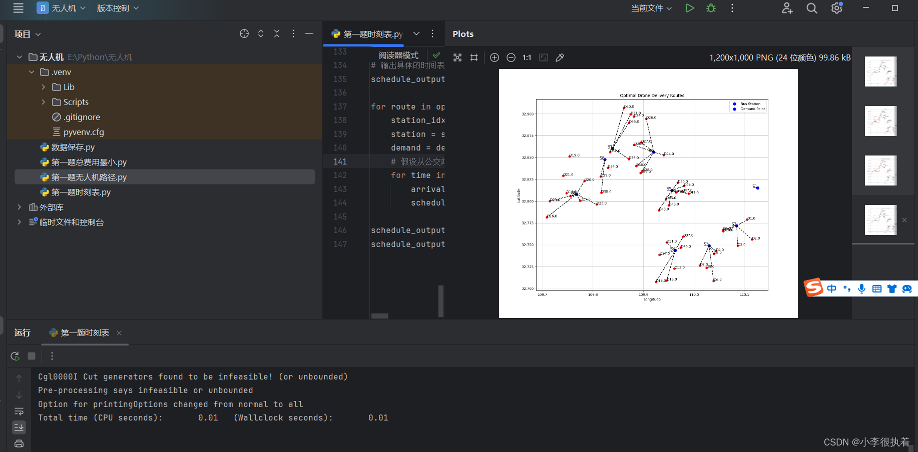
2. 可视化飞行路径和时间表
我们使用 Matplotlib 来绘制飞行路径和时间表。
- # 可视化飞行路径
- plt.figure(figsize=(10, 8))
-
- # 绘制公交站点
- for i, station in stations_data.iterrows():
- plt.plot(station['Longitude'], station['Latitude'], 'bo', markersize=8)
- plt.text(station['Longitude'], station['Latitude'], f'S{i+1}', fontsize=12, ha='right')
-
- # 绘制需求点
- for j, demand in demands_data.iterrows():
- plt.plot(demand['Longitude'], demand['Latitude'], 'ro', markersize=6)
- plt.text(demand['Longitude'], demand['Latitude'], f'D{demand["Demand_ID"]}', fontsize=10, ha='left')
-
- # 绘制最优路径
- for route in optimal_routes:
- station_idx, demand_idx, dist = route
- station = stations_data.iloc[station_idx]
- demand = demands_data.iloc[demand_idx]
- plt.plot([station['Longitude'], demand['Longitude']], [station['Latitude'], demand['Latitude']], 'k--')
-
- plt.xlabel('Longitude')
- plt.ylabel('Latitude')
- plt.title('Optimal Drone Delivery Routes')
- plt.legend(['Bus Station', 'Demand Point'])
- plt.grid()
- plt.show()
-
- # 输出具体的时间表
- schedule_output = []
-
- for route in optimal_routes:
- station_idx, demand_idx, dist = route
- station = stations_data.iloc[station_idx]
- demand = demands_data.iloc[demand_idx]
- # 假设从公交站出发的时间为公交车到达时间
- for time in bus_schedule['白河至仓上']:
- arrival_time = time + dist / bus_speed
- schedule_output.append((f'Station {station_idx+1}', f'Demand {demand_idx+1}', time, arrival_time))
-
- schedule_output_df = pd.DataFrame(schedule_output, columns=['Station', 'Demand', 'Departure Time', 'Arrival Time'])
- schedule_output_df
最终实现结果