缩放Logistic回归用于多GPU TPU训练

Logistic regression is a simple, but powerful, classification algorithm. In this blog post we’ll see that we can view logistic regression as a type of neural network.

Logistic回归是一种简单但功能强大的分类算法。在此博客文章中，我们将看到我们可以将逻辑回归视为一种神经网络 。

Framing it as a neural network allows us to use libraries like PyTorch and PyTorch Lightning to train on hardware accelerators (like GPUs/TPUs). This enables distributed implementations that scale to massive datasets.

将其构建为神经网络可以使我们使用PyTorch和PyTorch Lightning之类的库在硬件加速器(如GPU / TPU)上进行训练。这使分布式实现可以扩展到海量数据集。

In this blog post I’ll illustrate this link by connecting a NumPy implementation to PyTorch.

在此博客文章中，我将通过将NumPy实现连接到PyTorch来说明此链接。

I’ve added this highly scalable logistic regression implementation to the PyTorch Lightning Bolts library which you can easily use to train on your own dataset.

我已将此高度可扩展的逻辑回归实现添加到PyTorch Lightning Bolts库中，您可以轻松地使用它来训练自己的数据集。

Image for post — PyTorch Lightning PyTorch闪电

跟着 (Follow along)

All the code examples we’ll walk through can be found in this matching Colab notebook if you’d like to run the code in each step yourself.

如果您想自己在每个步骤中运行代码，则可以在此匹配的Colab笔记本中找到我们将遍历的所有代码示例。

为什么需要可伸缩的逻辑回归？ (Why do I need scalable logistic regression?)

Example using 8 GPUs to fit logistic regression.

使用8个GPU来拟合逻辑回归的示例。

Much like other ML libraries (e.g. Sci-kit Learn) this implementation will allow you to fit a logistic regression model in a few lines of code. Unlike other libraries, you’ll be able to train massive datasets on multiple GPUs, TPUs, or CPUs, across many machines.

与其他ML库(例如Sci-kit Learn)非常相似，此实现将使您可以在几行代码中拟合逻辑回归模型。与其他库不同，您将能够跨许多机器在多个GPU，TPU或CPU上训练大量数据集。

Beyond toy datasets with a dozen or so features, real datasets may have tens of thousands of features and millions of samples. At this scale, CPUs simply won’t do. Instead, we can leverage GPU and TPUs to turn days of training into minutes.

除了具有十二个左右特征的玩具数据集之外，真实的数据集可能还具有数万个特征和数百万个样本。在这种规模下，CPU根本不会这样做。相反，我们可以利用GPU和TPU将几天的培训变成几分钟。

For example, at the end of this tutorial we train on the full MNIST dataset containing 70,000 images and 784 features on 1 GPU in just a few seconds. And in fact, we have even tried ImageNet. Our logistic regression implementation can loop through all 1.3million images, each with 150,528 pixels (input features) in about 30 minutes on 2 GPUs (V100s).

例如，在本教程的最后，我们在短短几秒钟内就在1个GPU上训练了完整的MNIST数据集，其中包含70,000张图像和784个功能。实际上，我们甚至尝试了ImageNet。我们的逻辑回归实现可以在2个GPU(V100)上在30分钟内循环遍历所有130万张图像，每个图像具有150,528像素(输入功能)。

逻辑回归作为基线 (Logistic regression as a baseline)

No matter the complexity of your classification problem, it is always good practice to set a strong baseline using a logistic regression classifier. Even if you intend to use more complex approaches such as neural networks.

无论您的分类问题有多复杂，使用Logistic回归分类器设置一个严格的基线始终是一个好习惯。即使您打算使用更复杂的方法，例如神经网络。

The advantage of starting with a logistic regression baseline implemented in PyTorch, is that it makes it easy to swap out the logistic regression model with a neural network.

从PyTorch中实现的逻辑回归基线开始的优势在于，它可以轻松地用神经网络交换出逻辑回归模型。

逻辑回归回顾 (Logistic Regression Recap)

If you’re familiar with logistic regression feel free to skip this section.

如果您熟悉逻辑回归，请跳过本节。

We use logistic regression to predict a discrete class label (such as cat vs. dog), this is also known as classification. This differs from regression where the goal is to predict a continuous real-valued quantity (such as stock price).

我们使用逻辑回归来预测离散的类别标签(例如猫与狗)，这也称为分类。这与回归分析不同，回归分析的目标是预测连续的实值量(例如股票价格)。

In the simplest case of logistic regression, we have just 2 classes, this is called binary classification.

在逻辑回归的最简单情况下，我们只有2个类，这称为二进制分类 。

二进制分类 (Binary classification)

Our goal in logistic regression is to predict a binary target variable Y (i.e. 0 or 1) from a matrix of input values or features, X. For example, say we have a group of pets and we want to find out which is a cat or a dog (Y) based on some features like ear shape, weight, tail length, etc. (X). Let 0 denote cat, and 1 denote dog. We have n samples, or pets, and m features about each pet:

我们逻辑回归的目标是从输入值或特征X的矩阵预测二进制目标变量Y (即0或1)。例如，假设我们有一组宠物，我们要找出哪些是猫或狗( Y基于像耳朵的形状，重量，尾长等(某些功能) X )。设0代表猫，1代表狗。我们有n样本或宠物，每个宠物的m特征：

We want to predict the probability that a pet is a dog. To do so, we first take a weighted sum of the input variables — let w denote the weight matrix. The linear combination of the features X and the weights w is given by the vector z.

我们要预测宠物是狗的可能性。为此，我们首先对输入变量进行加权求和-令w表示权重矩阵。特征X和权重w的线性组合由向量z给出。

Next, we apply the sigmoid function to every element of the z vector which gives the vector y_hat.

接下来，我们将S型函数应用于z向量的每个元素，从而得出向量y_hat 。

The sigmoid function, also known as the logistic function, is an S-shaped function that “squashes” the values of z into the range [0,1].

S形函数 ，也称为逻辑函数 ，是一种S形函数，可将z的值“压缩”到[0,1]范围内。

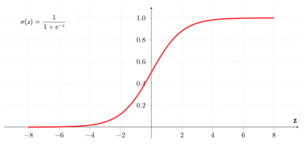
Since each value in y_hat is now between 0 and 1, we interpret this as the probability that the given sample belongs to the “1” class, as opposed to the “0” class. In this case, we’d interpret y_hat as the probability that a pet is a dog.

由于y_hat每个值现在都介于0和1之间，因此我们将其解释为给定样本属于“ 1”类而不是“ 0”类的概率。在这种情况下，我们将y_hat解释为宠物是狗的概率。

Our goal is to find the best choice of the w parameter. We want to find a w such that the probability P(y=1|x) is large when x belongs to the “1” class and small when x belongs to the “0” class (in which case P(y=0|x) = 1 — P(y=1|x) is large).

我们的目标是找到w参数的最佳选择。我们希望找到一个w ，使得当x属于“ 1”类时概率P(y=1|x)大，而当x属于“ 0”类时概率P(y=1|x)小(在这种情况下， P(y=0|x) = 1 — P(y=1|x)大)。

Notice that each model is fully specified by the choice of w. We can use the binary cross entropy loss, or log loss, function to evaluate how well a specific model is performing. We want to understand how “far” our model predictions are from the true values in the training set.

请注意，通过选择w可以完全指定每个模型。我们可以使用二进制交叉熵损失或对数损失函数来评估特定模型的执行情况。我们想了解我们的模型预测与训练集中的真实值有多“远”。

Note that only one of the two terms in the summation is non-zero for each training example (depending on whether the true label y is 0 or 1). In our example, when we have a dog (i.e. y = 1) minimizing the loss means we need to make y_hat = P(y=1|x) large. If we have a cat (i.e. y = 0) we want to make 1 — y_hat = P(y=0|x) large.

请注意，对于每个训练示例，求和中只有两项是非零的(取决于真实标签y是0还是1)。在我们的示例中，当我们有一条狗(即y = 1 )时，将损失最小化意味着我们需要使y_hat = P(y=1|x)大。如果我们有一只猫(即y = 0 )，我们想将1 — y_hat = P(y=0|x)大。

Now we have loss function that measures how well a given w fits our training data. We can learn to classify our training data by minimizing L(w) to find the best choice of w.

现在我们有了损失函数，可以测量给定w与我们的训练数据的拟合程度。我们可以学会通过最小化我们的训练数据进行分类L(w)找到的最佳选择w 。

One way in which we can search for the best w is through an iterative optimization algorithm like gradient descent. In order to use the gradient descent algorithm, we need to be able to calculate the derivative of the loss function with respect to w for any value of w.

我们可以搜索最佳w一种方法是通过迭代优化算法，例如梯度下降。 为了使用梯度下降算法，对于任何w值，我们都需要能够计算出相对于w的损失函数的导数。

Note, that since the sigmoid function is differentiable, the loss function is differentiable with respect to w. This allows us to use gradient descent, but also allows us to use automatic differentiation packages, like PyTorch, to train our logistic regression classifier!

注意，由于S形函数是可微的，所以损失函数相对于w是可微的。这不仅使我们能够使用梯度下降，而且使我们能够使用自动微分软件包(例如PyTorch)来训练逻辑回归分类器！

多类别分类 (Multi-class classification)

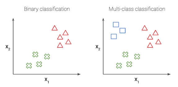
We can generalize the above to the multi-class setting, where the label y can take on K different values, rather than only two. Note that we start indexing at 0.

我们可以将以上内容概括为多类设置，其中标签y可以采用K不同的值，而不仅仅是两个。请注意，我们从0开始索引。

The goal now, is to estimate the probability of the class label taking on each of the K different possible values, i.e. P(y=k|x) for each k = 0, …, K-1. Therefore the prediction function will output a K-dimensional vector whose elements sum to 1, to give the K estimated probability.

现在的目标是估计类别标签采用K不同可能值(即，对于每个k = 0, …, K-1 P(y=k|x)的概率。因此，预测函数将输出一个K维向量，其元素之和为1，以给出K个估计概率。

Specifically, the hypothesis class now takes the form:

具体来说，假设类现在采用以下形式：

This is also known as multinomial logistic regression or softmax regression.

这也称为多项逻辑回归或softmax回归 。

A note on dimensions —above we are looking at one example only, x is a m x 1 vector, y is an integer value between 0 and K-1, and let w(k) denote a m x 1 vector that represents the feature weights for the k-th class.

关于尺寸的注释—以上仅是一个示例， x是mx 1向量， y是0到K-1之间的整数，并且w(k)表示mx 1向量，表示向量的特征权重第k个班级。

Each element of the output vector, takes the follow form:

输出向量的每个元素都采用以下形式：

This is known as the softmax function. The softmax turns arbitrary real values into probabilities. The outputs of the softmax function are always in the range [0, 1] and the summation in the denominator means all the terms add up to 1. Hence, they form a probability distribution. It can be seen as a generalization of the sigmoid function and in the binary case, the softmax function actually simplifies to the sigmoid function (try to prove this for yourself!)

这称为softmax函数 。 softmax将任意实数值转换为概率。 softmax函数的输出始终在[0，1]范围内，分母之和表示所有项加起来为1。因此，它们形成概率分布。可以看作是S型函数的一般化，在二进制情况下，softmax函数实际上简化为S型函数(尝试自己证明一下！)

For convenience, we specify the matrix W to denote all the parameters of the model. We concatenate all the w(k) vectors into columns so that the matrix W has dimension m x k.

为了方便起见，我们指定矩阵W表示模型的所有参数。我们将所有w(k)向量连接成列，以使矩阵W维数为mxk 。

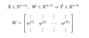
As in the binary case, our goal in training is to learn the W values that minimize the cross entropy loss function (an extension of the binary formula).

与二进制情况一样，我们的训练目标是学习使交叉熵损失函数(二进制公式的扩展)最小的W值。

现在进入神经网络 (Now onto neural networks)

We can think of logistic regression as a fully connected, single layer neural network followed by the softmax function.

我们可以将逻辑回归视为完全连接的单层神经网络，后跟softmax函数。

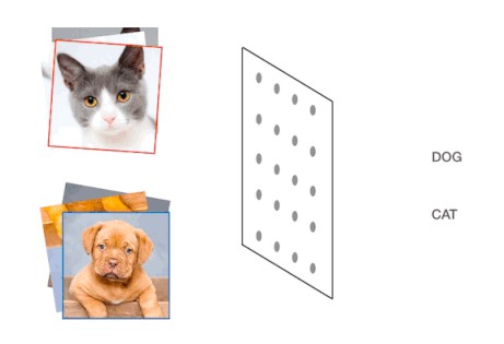
The input layer contains a neuron for each feature (and potentially one neuron for a bias term). In the binary case, the output layer contains 1 neuron. In the multi-class case, the output layer contains a neuron for each class.

输入层包含每个特征的神经元(对于偏置项可能包含一个神经元)。在二进制情况下，输出层包含1个神经元。在多类情况下，输出层包含每个类的神经元。

NumPy与PyTorch代码 (NumPy vs. PyTorch Code)

In fact, the traditional logistic regression and neural network formulations are equivalent. This is easiest to see in code — we can show that the NumPy implementation of the original formulas is equivalent to specifying a neural network in PyTorch. To illustrate, we’ll use examples from the Iris dataset.

实际上，传统的逻辑回归和神经网络公式是等效的。这是最容易在代码中看到的-我们可以证明原始公式的NumPy实现等效于在PyTorch中指定神经网络。为了说明，我们将使用Iris数据集中的示例。

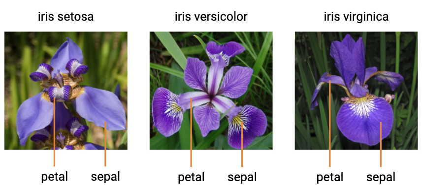
The Iris dataset is a very simple dataset to demonstrate multi-class classification. There are 3 classes (encoded as 0, 1, 2) representing the type of iris flower (setosa, versicolor and virginica). There are 4 real-valued features for the length and width of both the plant sepal and petal.

Iris数据集是一个非常简单的数据集，用于演示多类分类。有3个类别(编码为0、1、2)代表鸢尾花的类型(setosa，versicolor和virginica)。植物萼片和花瓣的长度和宽度都有4个实值特征。

Here is how we load and shuffle the Iris dataset using tools from the sci-kit learn datasets library:

这是我们使用sci-kit Learn数据集库中的工具加载和随机整理Iris数据集的方式：


import numpy as np
from sklearn.datasets import load_iris
from sklearn.utils import shuffle
 
 
# Load and shuffle Iris dataset
X, Y = load_iris(return_X_y=True)
X, Y = shuffle(X, Y, random_state=0)

Let’s inspect the dataset dimensions:

让我们检查数据集维度：

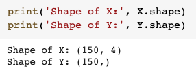
There are 150 samples — in fact we know there are 50 samples of each class. Now, let’s pick two specific examples:

有150个样本-实际上，我们知道每个类别有50个样本。现在，让我们选择两个具体示例：


# Let's look at the first two samples
x = X[0:2]
y = Y[0:2]

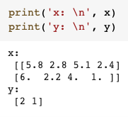
Above we see that, x has dimensions 2 x 4, because we have two examples and each example has 4 features. y has 2 x 1 values because we have two examples and each example has a label that could be 0, 1, 2 where each number represents the name of the class (versicolor, setosa, virginica).

在上面可以看到x尺寸为2 x 4 ，因为我们有两个示例，每个示例都有4个特征。 y具有2 x 1值，因为我们有两个示例，每个示例都有一个可能为0、1、2的标签，其中每个数字代表该类的名称(versicolor，setosa，virginica)。

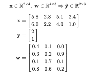
Now we’ll create the weight parameters that we want to learn w. Since we have 4 features for each of the 3 classes, the dimension of w has to be 4 x 3.

现在，我们将创建要学习w的权重参数。由于我们为3个类别中的每一个拥有4个特征，因此w的维数必须为4 x 3 。


# Initialize a random weight vector 
w = np.array([[0.4, 0.1, 0.0],
              [0.3, 0.2, 0.9],
              [0.1, 0.7, 0.1],
              [0.8, 0.6, 0.2]], dtype = np.float64)

Note: for simplicity, we’re looking only at the features and have not included a bias term here. Now we have,

注意：为简单起见，我们仅查看功能，此处未包含偏差术语。现在我们有了

在NumPy中学习w： (Learning w in NumPy:)

According to the logistic regression formula, we first compute z = xw. The shape of z is 2 x 3, because we have two samples and three possible classes. These raw scores need to be normalized into probabilities. We do this by applying the softmax function across each row of z.

根据逻辑回归公式，我们首先计算z = xw 。 z的形状为2 x 3，因为我们有两个样本和三个可能的类别。这些原始分数需要归一化为概率。我们通过在z每一行上应用softmax函数来做到这一点。


# Calculate the linear transformation
z = np.matmul(x, w)
 
 
# Apply softmax function
def softmax(z):
	return np.exp(z) / np.sum(np.exp(z), axis=1, keepdims=True)
 
 
y_hat = softmax(z)

Thus the final output y_hat has the same shape as z but now each row sums to 1 and each element of the row gives the probability of that column index as the predicted class.

因此，最终输出y_hat具有与z相同的形状，但是现在每一行的总和为1，并且该行的每个元素都将列索引的概率作为预测类。

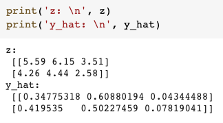
In the example above, the largest number in row 1 of y_hat is 0.6 which gives the second class label (1) as the predicted class. And for the second row, the predicted class is also 1, but with probability 0.5. In fact, in the second row, label 0 has also has a high probability of 0.41.

在上面的示例中， y_hat第1行中的最大数字为0.6，这将第二个类别标签(1)作为预测类别。对于第二行，预测类别也是1，但概率为0.5。实际上，在第二行中，标签0也具有0.41的高概率。

在PyTorch中： (In PyTorch:)

Now let’s implement the exact same thing but in PyTorch.

现在，让我们在PyTorch中实现完全相同的事情。

First we’ll need to convert our NumPy arrays to PyTorch Tensors.

首先，我们需要将NumPy数组转换为PyTorch张量。


import torch
import torch.nn as nn
 
 
# Transform numpy arrays to tensors
x_tensor = torch.from_numpy(x)
w_tensor = torch.from_numpy(w)

Then define the linear layer and softmax activation function of the neural network.

然后定义神经网络的线性层和softmax激活函数。


lin_layer = nn.Linear(in_features=4, out_features=3, bias=False)
softmax = nn.Softmax(dim=1)

PyTorch automatically initializes random weights so I explicitly replace the weights with the same weight matrix that we used above.

PyTorch会自动初始化随机权重，因此我将权重显式替换为我们上面使用的权重矩阵。


# Use the same weight matrix from above
lin_layer.weight.data = torch.transpose(w_tensor, 0, 1)

Now we calculate the output of this one layer neural network and see that it’s exactly the same as above.

现在，我们计算出这一层神经网络的输出，并发现它与上面完全相同。


# Calculate output
z_tensor = lin_layer(x_tensor)
y_hat_tensor = softmax(z_tensor)

This step above is called the forward pass (calculating the outputs and loss) when training a neural network the learn the optimal W. It is followed by the backward pass. During the backward pass, we calculate the gradient of the loss with respect to each weight parameter using the backpropagation algorithm (essentially, the chain rule) (link). Finally, we use the gradient descent algorithm to update the values of each of the weights. This constitutes one iteration. We repeat these steps, iteratively updating the weights, until the model converges or some stopping criteria is applied.

当训练神经网络学习最佳W时，上述步骤称为正向传递 (计算输出和损耗)。随后是向后传递。 在反向传递期间，我们使用反向传播算法(本质上是链规则)(链接)来计算相对于每个权重参数的损耗梯度。最后，我们使用梯度下降算法来更新每个权重的值。这构成一个迭代。我们重复这些步骤，迭代地更新权重，直到模型收敛或应用了一些停止条件。

As you see, the outputs are the same whether you’re using NumPy or a neural network library like PyTorch. However, PyTorch uses tensor data-structures instead of NumPy arrays which are optimized for fast performance on hardware accelerators like GPUs and TPUs. Thus, this allows for a scalable implementation of logistic regression.

如您所见，无论您使用的是NumPy还是PyTorch之类的神经网络库，输出都是相同的。但是，PyTorch使用张量数据结构而不是NumPy数组，后者针对在GPU和TPU等硬件加速器上的快速性能进行了优化。因此，这允许逻辑回归的可扩展实施。

A second advantage of using PyTorch is that we can use automatic differentiation to efficiently and automatically calculate these gradients.

使用PyTorch的第二个优点是我们可以使用自动微分来高效，自动地计算这些梯度。

使用PyTorch避雷针 (Using PyTorch Lightning Bolts)

Although it’s simple to implement a simple logistic regression example as I just did, it becomes very difficult to distribute data batches and training on multiple GPUs/TPUs across many machines correctly.

尽管像我刚才那样实现一个简单的逻辑回归示例很简单，但是要在许多计算机上正确地在多个GPU / TPU上分发数据批和训练变得非常困难。

However, by using PyTorch Lightning, I have implemented a version that handles all of these details and released it in the PyTorch Lightning Bolts library. This implementation makes it trivial to customize and train this model on any dataset.

但是，通过使用PyTorch Lightning，我实现了处理所有这些详细信息的版本，并将其发布在PyTorch Lightning Bolts库中。此实现使在任何数据集上自定义和训练该模型变得轻而易举。

1.首先，安装螺栓： (1. First, install Bolts:)

pip install pytorch-lightning-bolts

2.导入模型并实例化： (2. Import the model and instantiate it:)


from pl_bolts.models import LogisticRegression
 
 
model = LogisticRegression(in_features=4, num_classes=3, bias=True)

We specify the number of input features, the number of classes and whether to include a bias term (by default this is set to true). For the Iris dataset, we would specify in_features=4 and num_classes=3. You can also specify a learning rate, L1 and/or L2 regularization.

我们指定输入要素的数量，类的数量以及是否包括偏差项(默认情况下，此设置为true)。对于Iris数据集，我们将指定in_features=4和num_classes=3 。您还可以指定学习率，L1和/或L2正则化。

3.加载数据，该数据可以是任何NumPy数组。 (3. Load the data, which can be any NumPy array.)

Let’s continue with the Iris dataset as an example:

让我们继续以鸢尾花数据集为例：


import pytorch_lightning as pl
from pl_bolts.datamodules.sklearn_datamodule import SklearnDataset
from torch.utils.data import DataLoader
 
 
# Transform Sklearn/Numpy dataset to PyTorch (tensor) dataset
iris_dataset = SklearnDataset(X, Y)
 
 
# Put the PyTorch dataset into a DataLoader
iris_dataloader = DataLoader(dataset = iris_dataset,
                             batch_size = 10,
                             shuffle = True)

What you see above is how you load data in PyTorch using something called a Dataset and DataLoader. A Dataset is just a collection of examples and labels in PyTorch tensor format.

上面看到的是如何使用称为Dataset和DataLoader的东西在PyTorch中加载数据。数据集只是PyTorch张量格式的示例和标签的集合。

And a DataLoader is helps to efficiently iterate over batches (or subsets) of the Dataset. The DataLoader specifies things like the batch size, shuffle and data transforms.

DataLoader有助于有效地迭代数据集的批次(或子集)。 DataLoader指定诸如批处理大小，改组和数据转换之类的内容。

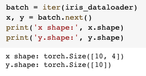
If we iterate over one batch in the DataLoader, we see that x and y both contain 10 samples, since we specified a batch size of 10.

如果我们在DataLoader中迭代一个批次，则可以看到x和y都包含10个样本，因为我们指定的批次大小为10。

DataModule:

数据模块：

In most approaches however we also need a training, validation and test splits of the data. With PyTorch Lightning, we have an extremely convenient class called a DataModule to automatically calculate these for us.

但是，在大多数方法中，我们还需要对数据进行训练，验证和测试拆分。使用PyTorch Lightning，我们有一个非常方便的类，称为DataModule ，可以为我们自动计算这些值。

We use the SklearnDataModule — input any NumPy dataset, customize how you would like your dataset splits and it will return the DataLoaders for you to feed to your model.

我们使用SklearnDataModule －输入任何NumPy数据集，自定义数据集拆分的方式，它将返回DataLoaders供您输入模型。


from pl_bolts.datamodules import SklearnDataModule
 
 
iris_dm = SklearnDataModule(X, Y, val_split=0.1, test_split=0.1, random_state=0)

A DataModule is nothing more than just a collection of a train DataLoader, validation DataLoader and test DataLoader. In addition to that, it allows you to fully specify and combine all your data preparation steps (like splits or data transforms) for reproducibility.

DataModule仅仅是火车DataLoader，验证DataLoader和测试DataLoader的集合。除此之外，它还允许您完全指定并组合所有数据准备步骤(例如拆分或数据转换)以提高可重复性。

I’ve specified splitting the data into 80% train, 10% validation, 10% test but can also pass in your own validation and test datasets (as NumPy arrays) if you would like to use your own custom splits.

我已经指定将数据拆分为80％训练，10％验证，10％测试，但是如果您想使用自己的自定义拆分，也可以传入自己的验证和测试数据集(作为NumPy数组)。

Say you have a custom test set with 20 samples and would like to use 10% of the training set for validation:

假设您有一个包含20个样本的自定义测试集，并希望使用训练集的10％进行验证：


# Use your own custom test dataset, use 10% of training data for validation
dm = SklearnDataModule(X, Y, 
                       x_test = np.random.rand(20, 4),
                       y_test = np.random.rand(20),
                       val_split=0.1,
                       shuffle=False)

Splitting your data is good practice but completely optional — just set either or both the val_split and test_split to 0 if you don’t want to use a validation or test set.

拆分数据是一种很好的做法，但完全是可选的-如果您不想使用验证或测试集，只需将val_split和test_split为0或两者都设置为0。


# No validation or test splits
dm = SklearnDataModule(X, Y, val_split=0, test_split=0)

4.训练模型 (4. Train the model)

Now that we have the data, let’s train our logistic regression model on 1 GPU. Training will start when I call trainer.fit (line 6). We can call trainer.test to see the model’s performance on our test set:

现在我们有了数据，让我们在1个GPU上训练逻辑回归模型。当我致电trainer.fit (第6行)时，训练将开始。我们可以调用trainer.test在我们的测试集中查看模型的性能：


# Build model
model = LogisticRegression(input_dim=4, num_classes=3, learning_rate=0.01)
 
 
# Fit the model
trainer = pl.Trainer(gpus=1)
trainer.fit(model, iris_dm.train_dataloader(batch_size=15), iris_dm.val_dataloader(batch_size=15))
 
 
# Look at test perfromance
trainer.test(test_dataloaders=iris_dm.test_dataloader(batch_size=15))
 
 
### Test set accuracy: 100%

Our final test set accuracy is 100% — which is only something we get to enjoy with perfectly separably toy datasets like Iris.

我们最终的测试集准确性为100％-只有像Iris这样完全独立的玩具数据集才可以享受到这一点。

Since I’m training this on a Colab notebook with 1 GPU, I’ve specified gpus=1 as an argument to the Trainer — however training on multiple hardware accelerators of any type is as simple as:

由于我是在带有1个GPU的Colab笔记本上进行训练的，因此我已将gpus=1指定为Trainer的参数-但是，使用多种类型的多种硬件加速器进行训练非常简单：

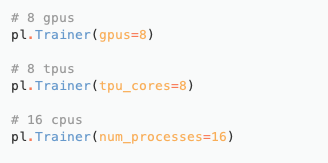
PyTorch Lightning deals with all the gritty details of distributed training behind the scenes so that you can focus on the model code.

PyTorch Lightning处理了幕后分布式培训的所有细节，因此您可以专注于模型代码。

训练完整的MNIST数据集 (Training on the full MNIST dataset)

Training on GPUs and TPUs is useful when running on large datasets. For small datasets, like Iris, hardware accelerators don’t make much of a difference.

在大型数据集上运行时，对GPU和TPU进行培训非常有用。对于Iris这样的小型数据集，硬件加速器的作用不大。

For example, the original MNIST dataset of handwritten digits contains 70,000 images of 28*28 pixels each. That means that the input feature space has dimension 784, and K = 10 different classes in the output space. In fact, implementations in Sci-kit Learn don’t use the original dataset, instead downsampled images of only 8*8 pixels are used.

例如，原始的MNIST手写数字数据集包含70,000张图像，每个图像28 * 28像素。这意味着输入要素空间的尺寸为784，输出空间中的K = 10个不同的类。实际上， Sci-kit Learn中的实现并不使用原始数据集，而是仅使用了8 * 8像素的降采样图像。

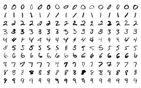
Given 785 features (28*28 + 1 for bias) and 10 classes, this means that our model has 7,850 weights that we’re learning (!).

给定785个特征(偏差为28 * 28 +1)和10个类，这意味着我们的模型拥有7,850个正在学习的权重(！)。


# Create the model instance
pixels_per_image = 28*28
model = LogisticRegression(input_dim=pixels_per_image, num_classes=10, learning_rate=0.01)

Bolts conveniently has a MNISTDataModule that downloads, splits and applies that standard transforms like image normalization to the MNIST digit images.

螺栓方便地具有MNISTDataModule ，可下载，拆分和应用该标准转换，例如将图像归一化到MNIST数字图像。


from pl_bolts.datamodules import MNISTDataModule
 
 
mnist_dm = MNISTDataModule(os.getcwd()) # default val split is 5000
 
 
# Download the MNIST dataset
mnist_dm.prepare_data()

Again we train using 1 GPU and see that the final test set accuracy (on 10,000 unseen images) is 92%. Pretty impressive!

再次，我们使用1个GPU进行训练，并看到最终测试集的准确性(在10,000张看不见的图像上)为92％。令人印象深刻！


# Fit the model
trainer = pl.Trainer(gpus=1, progress_bar_refresh_rate=0)
trainer.fit(model, mnist_dm.train_dataloader(), mnist_dm.val_dataloader())
 
 
# Calculate the test set accuracy
result = trainer.test(model, mnist_dm.test_dataloader()
 
 
### Test set accuracy: 92%

扩大规模 (Scaling even bigger)

Given the efficiency of PyTorch and the convenience of PyTorch Lightning, we could even scale this logistic regression model to train on massive datasets, like ImageNet, containing millions of samples.

鉴于PyTorch的效率和PyTorch Lightning的便利性，我们甚至可以扩展此逻辑回归模型，以对包含数百万个样本的海量数据集进行训练，例如ImageNet。

If you’re interested in learning more about Lightning/Bolts I’d recommend looking at these resources:

如果您有兴趣了解有关闪电/螺栓的更多信息，建议您查看以下资源：

如何开始 (How to start)

Hopefully this guide showed you exactly how to get started. The easiest way to start is to run the Colab notebook with all the code examples we’ve looked at already.

希望本指南向您确切地介绍了如何入门。最简单的开始方法是使用我们已经看过的所有代码示例来运行Colab笔记本。

You can try it yourself by just installing bolts and playing around! It includes different datasets, models, losses and callbacks you can mix and match, subclass, and run on your own data.

您只需安装螺栓并四处游玩即可自己尝试！它包括不同的数据集，模型，损失和回调，您可以混合和匹配，子类化并在自己的数据上运行。

pip install pytorch-lightning-bolts

Or check out PyTorch Lightning Bolts.

或查看PyTorch防雷螺栓。

翻译自: https://towardsdatascience.com/scaling-logistic-regression-for-multi-gpu-tpu-training-b4898d5049ff